
| Figure 10-1. Block diagram illustrating slip and rake for a normal fault. Points A and B were originally adjacent. |
In many situations, faults may be considered as roughly planar features. Thus, the orientation of a fault is given by strike and dip. Based on the fault's dip and the relative movement of blocks along the fault, four basic kinds of faults are recognized.
Slip is the actual measurement of displacement between two originally adjacent points in the fault plane—see Fig. 10-1. The net slip or total slip is the direct distance between the two points measured in whatever units are convenient: feet, m, miles, or km. Net slip is made up of two components: strike slip and dip slip, which are measured parallel to the strike and dip of the fault plane. The angle formed between the net-slip vector and strike of the fault is called rake.
|
| Figure 10-1. Block diagram illustrating slip and rake for a normal fault. Points A and B were originally adjacent. |
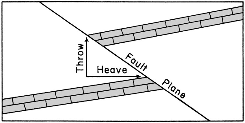
| Figure 10-2. Cross section of a thrust fault illustrating measurement of throw and heave on the top of a limestone bed. Cross section is vertical and oriented perpendicular to the fault strike. |
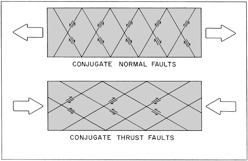
| Figure 10-3. Cross sections showing idealized normal and thrust conjugate fault patterns. Large arrows show overall sense of horizontal displacement. |
Another category of fault patterns involves the rotation of fault blocks during displacement. A single set of normal fault blocks which undergo rotational tilting results in overall thinning and lengthening of a rock mass—see Fig. 10-4. Tilted fault blocks produce crustal extension, so they often accompany conjugate normal faulting. Stacked or imbricated thrusts also undergo rotational tilting during thrusting—see Fig. 10-5. This style of faulting may accompany conjugate thrusts and results in shortening and thickening of the rock mass.
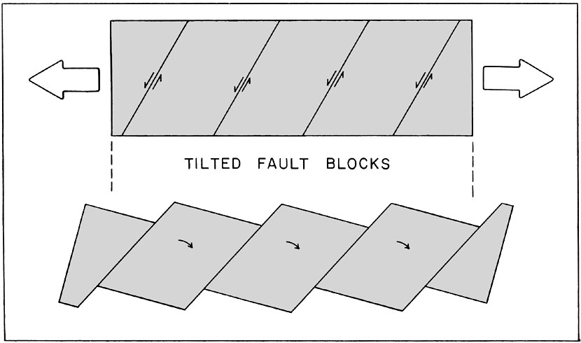
| Figure 10-4. Cross sections illustrating development of idealized tilted normal fault blocks. Large arrows indicate overall sense of horizontal displacement. |

| Figure 10-5. Cross sections illustrating development of idealized imbricated thrust blocks. Large arrow shows overall sense of horizontal displacement. |
The fault zone itself may possess one or more features, such as slickensides and striations, resulting from the grinding and abrasion of rock during movement. Fault gouge is a finely powdered rock debris; breccia consists of jumbled, angular stones broken from the fault walls. Under conditions of high pressure and temperature, a banded metamorphic rock called mylonite may develop. Mylonite consists of crushed rock debris strongly welded together with a fault-parallel foliation. Shearing in strata adjacent to the fault often results in small folds, called drag folds, whose orientation indicates the direction of slip.
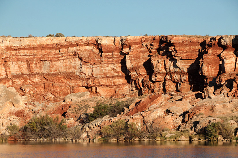
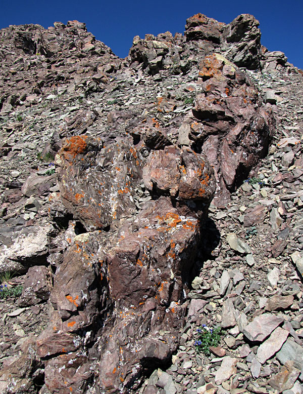
| Reverse fault with drag folding in Permian red beds with gypstone layers. Overview (left) and close-up shot (right); cliff is about 80 feet (~25 m) tall. Lea Lake, Bottomless Lakes State Park, New Mexico. | 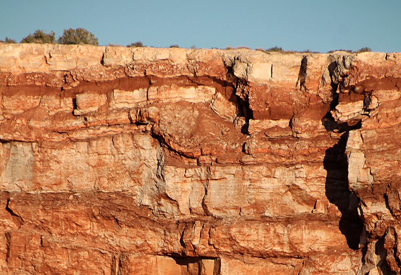
|
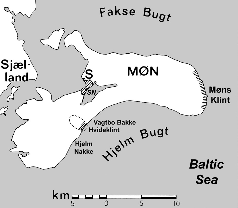 Figure 10-6. Locality map, Mřn, southeastern Denmark. S = City of Stege and SN = Stege Nor, a lagoon. Dashed line shows position of ice-shoved hill in which Hvideklint is cut. Adapted from Aber (1979).
| |
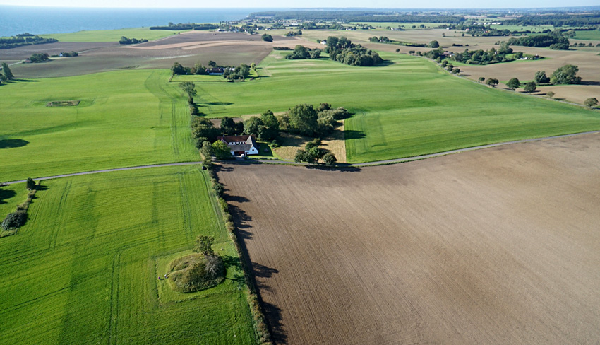
| Undulating terrain of ice-shoved hill inland from Hvideklint. Hill tops exceed 35 m (115 feet) above sea level. Kite aerial photograph looking southward by J.S. and S.E.W. Aber (2023). |
 Figure 10-7. Measured profile of Hvideklint section as it appeared in 1979. Note 2X vertical exaggeration; scale in m; adapted from Aber et al. (1989). | |
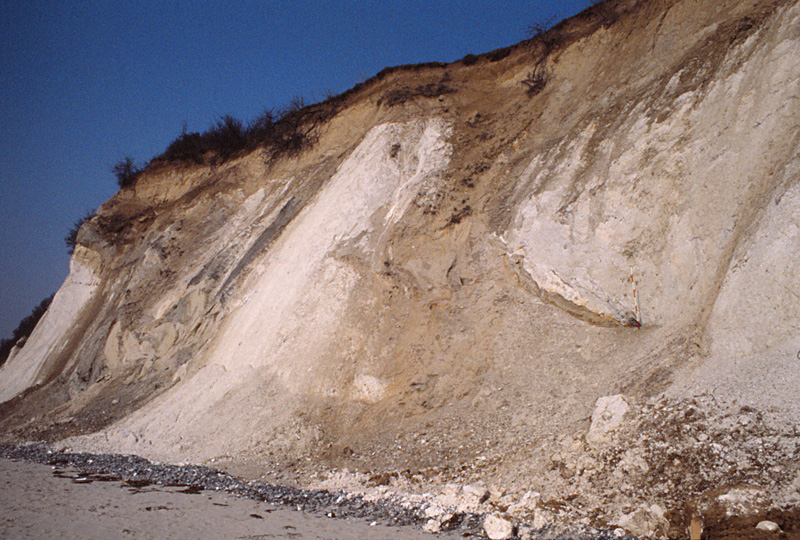
| Overview of a large chalk raft (left) that is pushed over deformed drift and chalk along a major thrust fault next to the scale pole. Between meters 830 and 900 of the measured section. Chalk resting on smeared glacial sediment (right). Note thin slivers of glacial sediment sheared into base of chalk mass. Fault #5 in Table 10-2. | 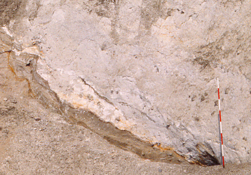 |
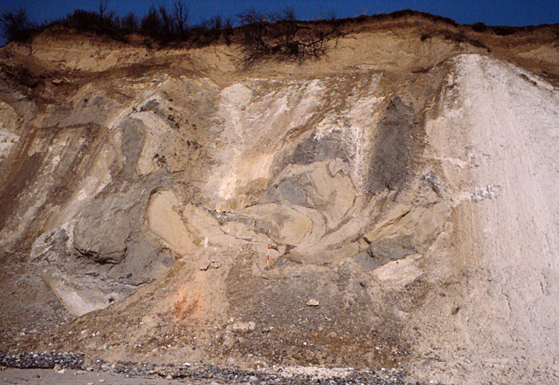
| Highly folded, faulted, and contorted till, sand, and gravel are "sandwiched" between chalk bodies (left). Between meters 860 and 900 of the measured section. Scale pole at center is marked in 20-cm stripes. Western end of Hvideklint (right) displays extremely stretched and folded chalk-till mélange. | 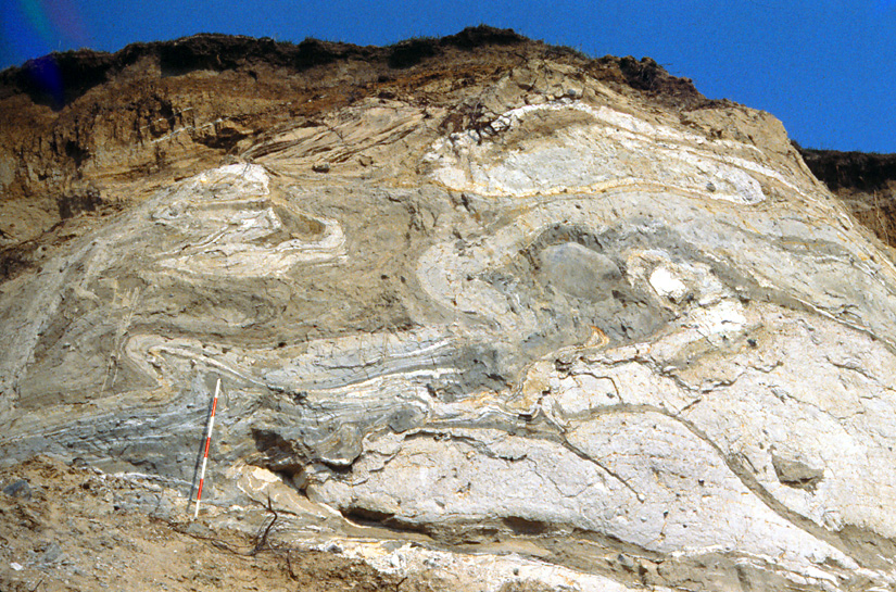
|
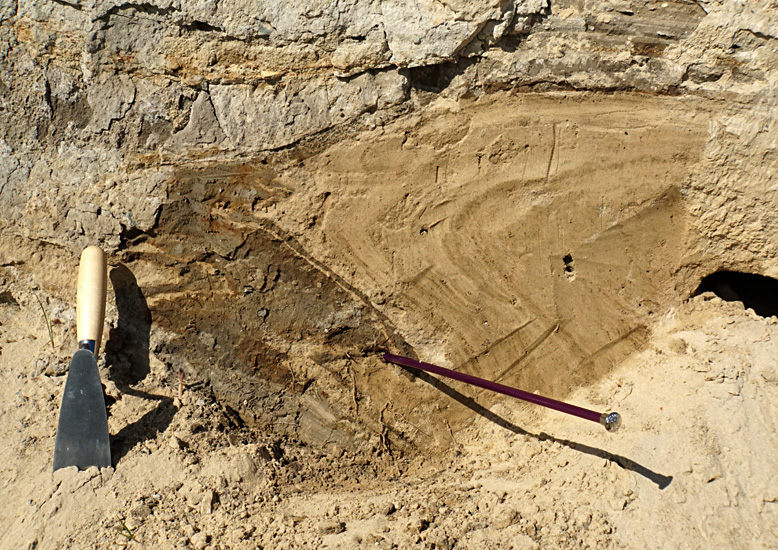
| Folded sand within till (left). Knitting needle indicates the fold axis. Overturned fold of sand (right) with a till core and expanded upper limb in silty fine sand (swallow nests). | 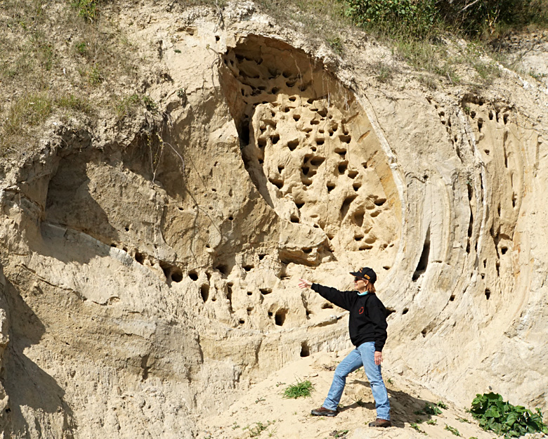 |

| Isoclinal, nearly recumbent fold of sand and till. Overview (left) and close-up shot (right). Knitting needle (^) indicates the fold axis. Fold #19 in Table 10-1. | 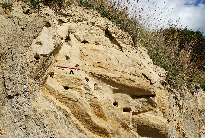
|
| Folds | Trend/Plunge |
|---|---|
| 1. Pinched syncline overturned to SW | 130/10 |
| 2. Isoclinal fold | 120/06 |
| 3. Small recumbent fold | 162/10 |
| 4. Overturned tight synform | 118/06 |
| 5. Tight synform | 128/12 |
| 6. Tight fold in clay bed | 110/00 |
| 7. Isoclinal fold in sand | 164/00 |
| 8. Isoclinal fold in sand | 138/06 |
| 9. Isoclinal fold in sand | 342/40 |
| 10. Small open fold parallel to large overturned fold | 290/08 |
| 11. Recumbent isoclinal fold of till in sand | 300/08 |
| 12. Kink fold on limb of overturned fold | 125/10 |
| 13. Large overturned fold | 116/06 |
| 14. Overturned fold in chalk-banded till | 265/40 |
| 15. Small overturned and recumbent fold | 330/20 |
| 16. Small overturned and recumbent fold | 255/10 |
| 17. Small overturned fold in sand | 155/10 |
| 18. Small overturned fold in sand | 155/15 |
| 19. Large isoclinal fold in sand | 85/06 |
| 20. Large overturned fold with bulbous limb | 135/10 |
| 21. Large overturned fold in flint breccia | 135/14 |
| 22. Drag fold in till along chalk/till fault | 260/26 |
| Faults and fold limb | Strike/dip |
|---|---|
| 1. Small normal fault | 118/62 |
| 2. Normal fault | 118/68 |
| 3. Small normal fault | 100/58 |
| 4. Small thrust fault | 296/16 |
| 5. Banded thrust zone below large chalk mass | 342/32 |
| 6. Limb of large syncline in chalk | 110/40 |
| 7. Reverse fault between chalk and till | 130/75 |
The example shows two plates (A and B) separated
by spreading ridges and transform faults, and rotating about an
axis running through the center of the Earth—see Fig. 11-1. The rotation axis
intersects the surface at two points called poles of rotation on
opposite sides of the globe. The positions of the poles of
rotation are specified by latitude and longitude coordinates. As
plates may move in any direction, rotation axes may occur in all
orientations. Hence, rotation poles may be located anywhere on
the surface of the Earth.
A series of great circles drawn through the rotation poles
for any pair of plates form so-called meridians or longitudes of
rotation (fig. 11-1). Likewise, a series of concentric small
circles and an equator constructed around the rotation poles are
called circles or latitudes of rotation. Latitudes and longitudes of rotation are useful for analyzing plate motion, but they should not be confused with the standard latitude and longitude
lines shown on maps. The latitudes and longitudes of rotation
are related solely to the poles of rotation and, thus, may be
positioned in any orientation on the Earth's surface.
Angular velocity is typically symbolized as wAB, where the subscripts (A and B) refer to the two plates involved, with the first one assumed to be fixed in position for purposes of calculations. WAB reads literally, the angular velocity with respect to A of B. To determine the sense of rotation—clockwise or counterclockwise—the so-called right-hand rule is used. The fingers of an imaginary right hand positioned at the center of the Earth with the thumb pointing northward along the axis of rotation would curl in a positive or clockwise direction.
In the example (fig. 11-1), plate A is assumed to be stationary, while plate B is moving toward the southeast; according to the right-hand rule plate B is moving clockwise. For example, wAmAf, the angular velocity with respect to America of Africa, is +0.37° per million years (LePichon 1968).
The nature of the boundary between two plates depends on the
position of the boundary relative to the poles of rotation for
the pair of plates. Where the boundary is parallel to latitudes
of rotation, a transform fault is formed (fig. 11-1), and the
plates slide past each other side by side. Two plates which are
diverging develop a ridge or spreading boundary which is parallel
to a longitude of rotation.
The positions of the rotation poles for a pair of plates are easily found by reference to spreading ridge segments or transform faults developed along their common boundary. Consider, for example, that portion of the Mid-Atlantic Ridge separating North America and Africa. Great circles drawn parallel to ridge segments and perpendicular to transform faults all intersect at the poles of rotation. In this case, the poles of rotation are located at 58° N, 37° W and 58° S, 143° E (LePichon 1968).
Given w and the poles of rotation for a pair of plates, one
of which is assumed fixed in position, the linear velocity at any
point on the mobile plate may be found. The maximum linear
velocity occurs on the equator of rotation, which represents
a great circle of 40,000 km circumference. One degree of a great
circle equals approximately 111 km. Continuing our example, wAmAf = 0.37° or 41 km per million years (4.1 cm per year) on the equator of rotation. Other points on the plate move at slower linear velocities depending on their latitudes of rotation.
At high latitudes, the magnetic field has a steep inclination, and at low latitudes it has a shallow inclination (Fig. 12-1). In fact, there is a strict relationship between latitude and inclination—see Fig. 12-2.
The NRM of Cenozoic rocks is generally parallel to the
modern (or reversed) geomagnetic field. However, older rocks
have NRM significantly different in orientation from the modern
field. For rocks of a given age and continent, the apparent
position of the paleopole may be calculated, and when paleopoles
representing each geologic period are plotted, a progressive
movement or wandering of the pole through time may be seen. The
path of apparent pole movement is called a polar wandering curve.
The term polar wandering is, unfortunately, somewhat misleading. It does not mean that the Earth's magnetic field has actually wandered, for the polar wandering curves of each continent are different. In fact, the Earth's magnetic field has remained more-or-less constant, aside from reversals and minor magnetic drift, while the continents have migrated independently of each other through time. Thus, polar wandering curves actually represent the paths of continental drifting.
The position of the magnetic paleopole may be determined
from NRM declination and inclination of samples from a specific
site—see Fig. 12-3. Declination is assumed to be approximately
parallel to the paleomeridian, and inclination is used to calculate the paleolatitude (or paleocolatitude). The various geometric elements necessary to solve for paleopoles are:
If the sample rocks in the example are, say, Late Eocene (38 million BP) in age, then the average minimum rate of polar wandering would be: 3774 km/38 million years, or approximately 10 cm per year. In reality, the pole has not wandered, rather the sample rocks have been displaced from their site of origin. However, this displacement may involve both rotational and translational movements, and so it is not always possible to determine the actual distance of rock movement without additional paleomagnetic information.
Note: the paleopole equations do not distinguish magnetic polarity. Be sure to pay attention to positive and negative values. If PL is negative, then PC also is negative, such that PL + PC = -90°. Your resulting answers may turn out in the northern hemisphere (positive Lp) or in the southern hemisphere (negative Lp). Round off PL, PC, Lp, and Mp values to nearest whole degree.
Some calculations in question 1 produce southern hemisphere paleopoles. These must be converted into equivalent northern hemisphere poles to plot on the graph. The conversion procedure is simple: (1) drop the negative sign from latitude and (2) subtract (or add) 180° to Mp.
Connect paleopoles with a smooth line reaching up to the North Pole to construct the North American polar-wandering curve. To orient yourself to the present position of the United States on this graph, plot the location of Denver, Colorado: 40° N, 105° W.
11. GEOMETRY OF PLATE MOTION
Plate rotation
The movement of rigid lithospheric plates over the surface of the Earth is properly understood in terms of spherical geometry. The Earth may be treated as a perfect sphere with a circumference of roughly 40,000 km for purposes of plate-motion calculations. The relative motion of any two plates which meet along a common boundary—trench, mid-ocean ridge, or transform fault—represents a rotation of the plates about an imaginary axis running through the center of the Earth.
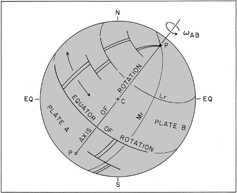
Figure 11-1. Geometric elements of plate motion. Spreading ridges shown by double lines; transform boundaries are single lines. Lr = latitude of rotation; Mr = longitude (meridian) of rotation; C = center of Earth; P = pole of rotation.
Linear and angular velocity
Velocity of plate movement may be described in two manners: (1) linear or surface velocity at a point and (2) angular velocity of rotation about the axis. Linear velocity is the more familiar, such as miles or km per hour, with plate velocities usually given in cm per year. However, linear velocity is not constant for a plate, being less near the poles of rotation and greater near the equator of rotation. For this reason, it is preferable to measure plate velocity as an angular movement about the rotation axis in degrees or radians per million years. Angular velocity is constant throughout the plate.

Age of North Atlantic oceanic crust. NOAA
image obtained from Wikimedia Commons.
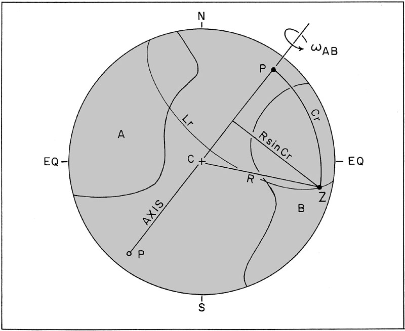
Figure 11-2. Angular and linear velocity of a point (Z) on a plate (B). Cr = colatitude of rotation; R = radius of Earth.
For instance, a point on the 35° latitude of rotation (Cr = 55°) would move at 82 percent of the equatorial linear velocity; at 65° (Cr = 25°), only 42 percent of the equatorial velocity occurs. Linear velocity is zero at the poles of rotation, which simply turn in a circle without moving in position.
Lr = latitude of rotation.
Cr = colatitude of rotation (Cr + Lr = 90). Haversine function
In order to make the conversion between angular and linear
velocities for any given point on a plate, it is necessary to
know the angular distance (colatitude) between the point and the
nearest pole of rotation. This difficult problem in spherical
trigonometry is simplified by using the haversine (meaning half
of the versed sine) function.
The haversine value increases from 0 to 1 for angles of 0° to
180°; it is always positive and never greater than 1.
Table 11-1 gives natural haversine values for 0° to 180°.
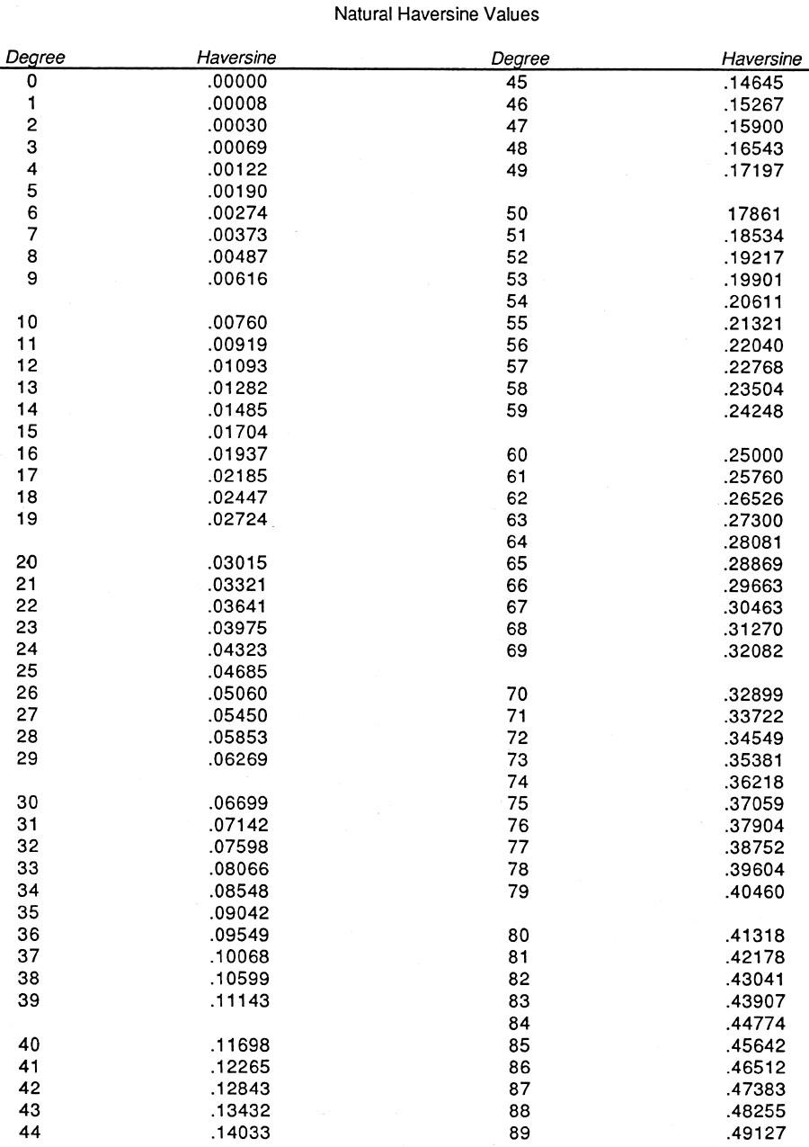
Table 11-1. Haversine
values for 0° to 180°.
The angular distance (D) between any point on the plate and
the nearest pole of rotation is equivalent to the colatitude of
rotation (Cr). Thus, a general formula for relating linear and
angular velocities of a plate is:
L = latitudes of points 1 and 2.
Md = difference in longitudes between points 1 and 2 (using the lesser of M1 - M2 or M2 - M1).
w = angular velocity in degrees per million years.
Cr = colatitude of rotation for the point (= D, between the point and the nearest pole of rotation). Problem
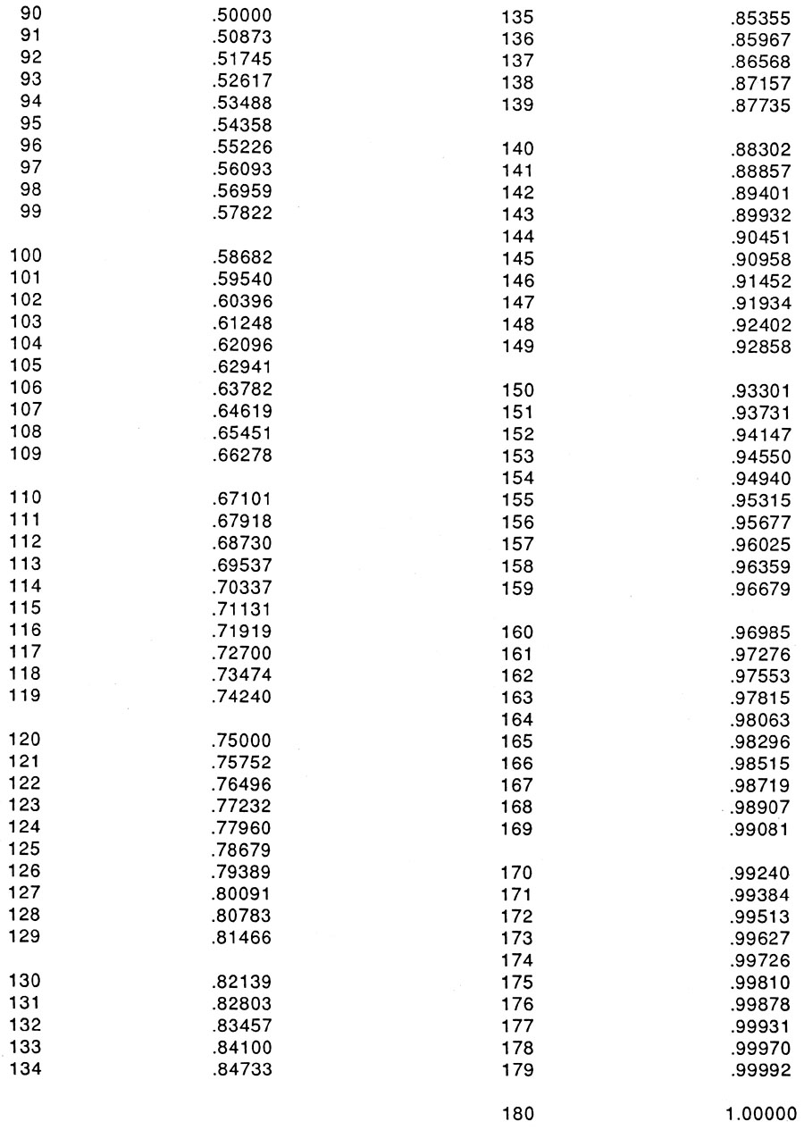
The Mid-Atlantic ridge in the vicinity of Iceland (see above) separates the North American and European plates. The American-European pole of rotation is located at 78° N, 102° E (LePichon 1968). Active seafloor spreading is taking place along the Reykjanes ridge—see Fig. 11-3. A hot spot is presently located beneath east-central Iceland at about 65° N, 17° W, as shown by high levels of volcanic and seismic activity and by a pronounced gravity anomaly.
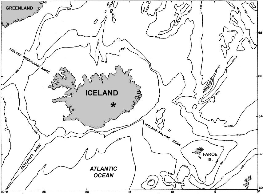
Figure 11-3. Map of the Iceland-Faroe region of the North Atlantic. Position of the North American-European plate boundary shown by Reykjanes Ridge; approximate position of Iceland hot spot shown by asterisk. Depth contours on seafloor in fathoms (100 f = 183 m).
 Volcanic features in Iceland
Eldgjá scoria deposit (left) in south-central Iceland. The scoria was erupted from a fissure vent about 1000 years ago. Laki lava flows (right), southeastern Iceland. The eruption at Lakagígar in 1783-84 was the largest such historical event in the world. The rough lava flows are now covered by soft moss, but the terrain remains largely impassable today.
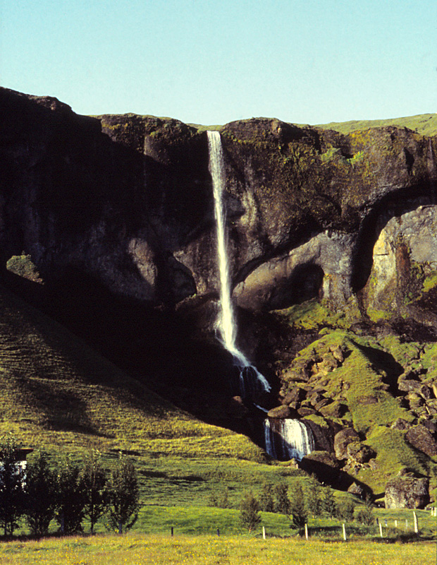
Relatively old Neogene basalt flows (>3 million years old) in southeastern Iceland. Water fall at Fagifoss (left), and cliff behind the Smyrlabjörg farm (right). Photographs © J.S. Aber.

 Volcanoes of Iceland.
 Faroe Islands geology
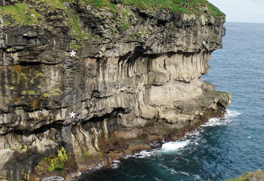
Cliff section at Gjógv at the northern end of Streymoy Island. Overview (left); note people at lower right for scale. Closer shot (right) showing a vertical dike (*) that cuts through layers of basalt and pyroclastic strata of the Malinstindur Formation (middle basalt series).

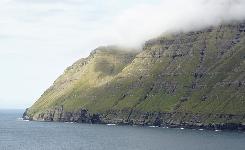
Villingadalsfjall mountain and village of Vidareidi on the island of Vidoy, northernmost Faroe Islands. Overview (left); mountain peak is 841 m above sea level. Closer shot (right) showing basalt lava flows on coastal cliff and steep hill side. Enni Formation (upper basalt series).
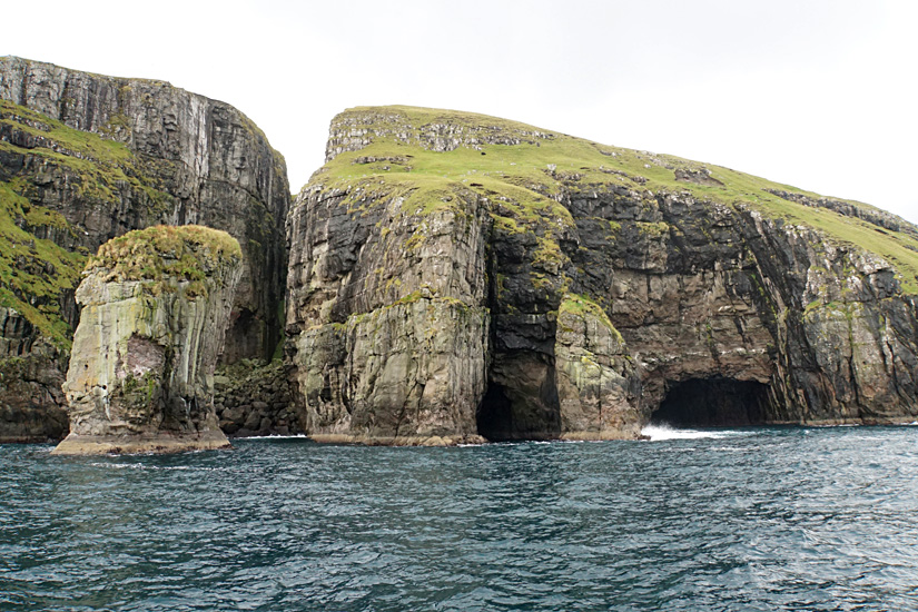
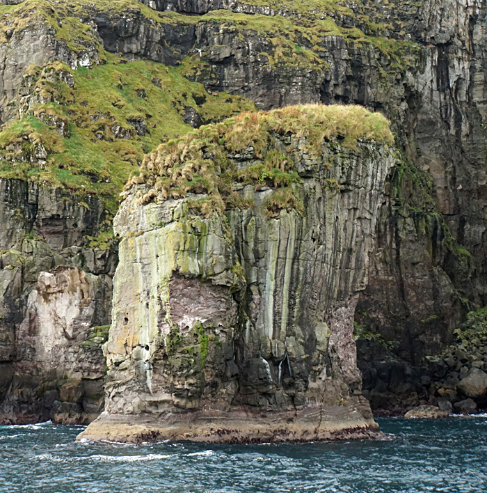
Cliff, cleft, sea caves, and isolated pillar (left) on the eastern coast of Vágar. Close-up view of pillar (right) shows well-developed columnar jointing in thick basalt flows of the Malinstindur Formation (middle basalt series).
Photographs © J.S. Aber.
 Geology of the Faroe Islands.
Calculations
References
12. POLAR WANDERING
Natural remnant magnetism
All iron-bearing rocks may acquire at the time of their
formation or sometime later a magnetic field, called natural
remnant magnetism (NRM), which is roughly parallel with the
Earth's magnetic field at that time. Thus, ancient rocks may
serve as a kind of "fossil compass." This is of particular
usefulness in plate tectonics for establishing the past positions, movements,
and configurations of continental masses. Rocks may acquire NRM
in several manners.
Not all rocks, of course, retain a useable NRM. In some
cases, the age of the rock may be known, but the time when NRM
was acquired may be indefinite. Later metamorphism and diagenesis could overprint a secondary NRM. Weathering and lightning strikes may also alter the fossil NRM of surface rocks. In most paleomagnetic laboratories, NRM is measured using a spinner magnetometer. Samples are subjected to stepwise demagnetization in order to determine the consistency and reliability of NRM measurements from particular rocks.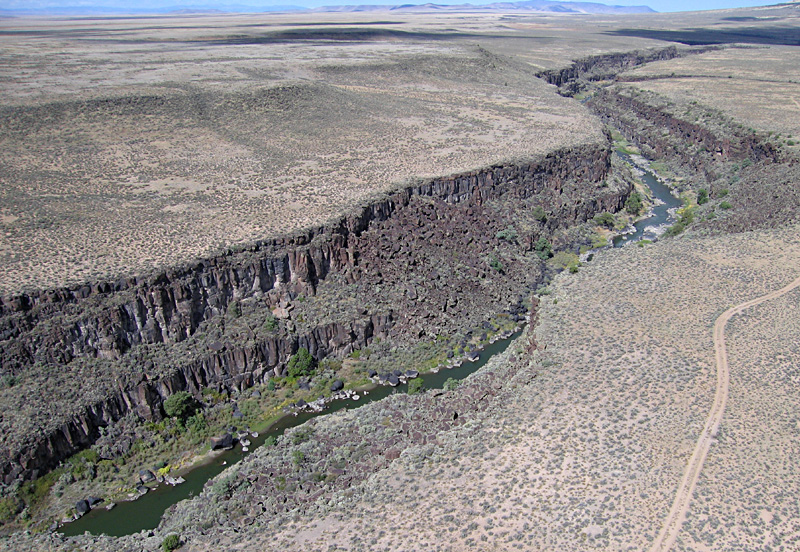
The Río Grande has eroded a deep canyon through thick lava flows of the Servilleta Basalt, which was erupted in the Taos Plateau between 4.8 and 2.8 million years ago (Bauer 2011). The canyon is about 200 feet (60 m) deep here; note the prominent columnar jointing. San Luis Valley of northern New Mexico. Kite aerial photograph.
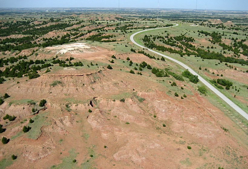
Permian red shale and siltstone of the Flower-pot Shale are eroding to form badlands in the foreground. The light-colored butte to left is capped by the Medicine Lodge Gypsum of the Blaine Formation. Red Hills of south-central Kansas. Kite aerial photograph.
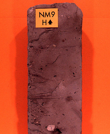
Split drill-core sample of glacial till from a buried valley in northeastern Kansas. Such till preserves a weak, but stable remnant magnetism. Core is approximately 3 inches (7˝ cm) in diameter. All photos © J.S. Aber. Earth's magnetic field
The Earth behaves basically as a large bar-magnet generating a dipole field—see Fig. 12-1. The orientation of the Earth's magnetic field at any point is determined by two measurements: declination and inclination. Declination (= trend) is defined as the angle between magnetic north and true north. The modern magnetic north pole is located in Arctic Canada, and its position drifts slowly from year to year. This magnetic drift is insignificant over geological time spans, and the average position of the magnetic pole is thought to coincide with the geographic pole.
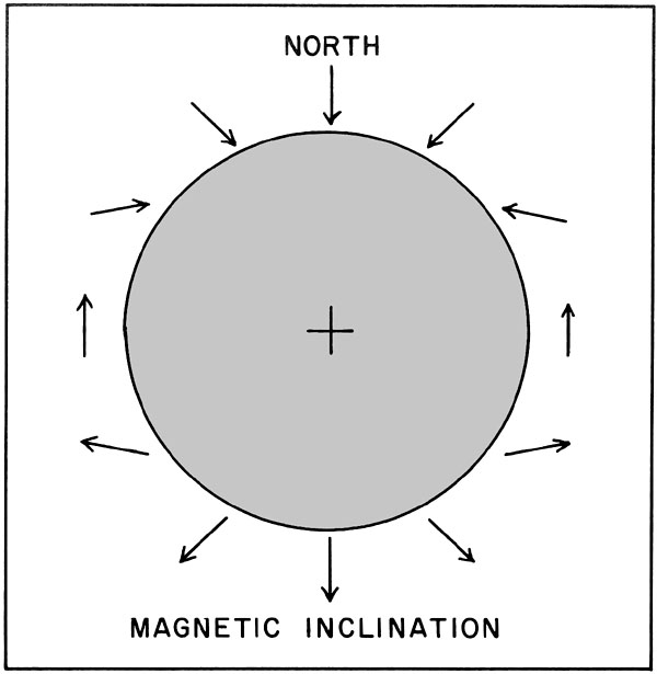
Figure 12-1. Dipole magnetic field of the Earth with magnetic inclination shown by arrows.
C = colatitude of site relative to modern pole.
M = meridian (longitude: 0° to 360°) of site.
I = inclination of magnetic field at site.
D = declination of magnetic field at site.
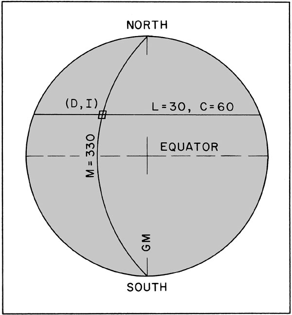
Figure 12-2. Geometric elements of modern geomagnetic field. At the site indicated by the small box, I = +49°. GM = Greenwich Meridian.
Polar wandering
The inclination of NRM in an ancient rock is a direct
indicator of the paleolatitude at which the rock originated.
This is the case assuming the original horizontal position of the
rock may be ascertained and the NRM is found to be stable to a
high level of demagnetization. In itself, determination of
paleolatitude is of great usefulness for paleogeographic reconstructions. For example, paleomagnetic evidence indicates that North America was astride the equator during most of the Paleozoic (Irving 1964). This is consistent with widespread Paleozoic coal beds, carbonate reefs, evaporites, and other low-latitude
indicators in the sedimentary record of the continent. NRM data
may be further used to calculate the positions of paleopoles.
L = latitude of sample site.
C = colatitude of sample site.
PL = paleolatitude: tan(I) = 2tan(PL).
PC = paleocolatitude: cot(I) = 2cot(PC).
Lp = latitude of paleopole (modern coordinates).
Mp = meridian of paleopole (modern coordinates).
I = inclination of NRM of sample rocks.
D = declination of NRM of sample rocks.
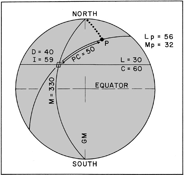
Figure 12-3. Geometric elements of paleomagnetic field and location of paleopole at point P. The dotted line from the North Pole to the paleopole shows the polar wandering curve. GM = Greenwich Meridian; sample site shown by small box.
In this example:
During the time since the NRM of rocks at the sample site
formed, the pole appears to have wandered a considerable distance
from the North Pole toward the south (Fig. 12-3). The rate of
apparent polar wandering depends on length of the polar wandering
curve (distance from paleopole to modern pole) versus age of the
sample rocks. The shortest possible polar wandering curve is
along a meridian (Fig. 12-3), and its distance is simply the
colatitude of the paleopole times 111 km per degree; for this
example: 90 - 56 = 34°, or 3774 km. This assumes the
paleopole has shifted position N-S along a meridian, which is
probably not the case, so the actual polar wandering curve is
likely longer.
Lp = arc sin (.8296) = 56° N.
Mp - M = arc sin (.88056)
Mp = 62 + 330 = 392°, or 32° E. Problem
Table 12-1 presents paleomagnetic data for rocks of six ages from the contiguous United States—see Fig. 12-4 (below). From this information, answer the following questions.
Taken from Irving (1964).Formation Age L M D I
1. Green River Formation Eocene
40 252 345 65
2. Granite, Sierra Nevada Cretaceous
38 240 335 61
3. Supai Formation Permian
35 250 150 11
4. Barnett Formation Carboniferous
31 261 322 -5
5. Clinton Iron Ore Silurian
34 273 143 19
6. Juniata Formation Ordovician
40 281 131 26

Figure 12-4. Map of the contiguous United States showing locations of samples sites for paleomagnetic data (Table 12-1).

Polar-projection graph. The center of the graph represents the geographic North Pole; Greenwich Meridian is the “0” radial line. Plot Lp and Mp coordinates for paleopoles. Print at full size. References
![]()
![]() Return to Table of Contents.
Return to Table of Contents.
