
| Figure 7-1. Schmidt stereographic projection. Print out a full-sized version for the problem below. |
|
| Figure 7-1. Schmidt stereographic projection. Print out a full-sized version for the problem below. |
The Schmidt stereonet has one important advantage—it preserves area. Therefore, the density of plotted data may be analyzed. In many situations, dozens or even hundreds of measurements of linear or planar features may be made, and all the data could be plotted on a single Schmidt stereonet to display the over all structural pattern.
Petrofabric is normally related to the larger structures formed at the same time the fabric developed. For example, lineation may parallel fold axes, or foliation may parallel fold axial planes. The petrofabric of a rock reflects the internal changes or strain that occurred within the rock body during deformation (further discussion in exercise 9). Thus, petrofabric analysis could give important additional information for overall structural interpretation.
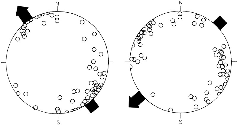
| Figure 7-2. Representative long-axis till-fabric plots on the Schmidt stereonet. Till fabric parallel with ice movement (left), and till fabric transverse to ice movement (right). From Nielsen and Houmark-Nielsen (1983, figs. 218 and 220). |
| Till exposed in a drumlin at Galway, Ireland. Overview (left) and close-up shot (right). A classic example of boulder-clay in which pebbles and cobbles of limestone appear to float in a fine-grained matrix. Long axes of larger clasts could be used to determine the till fabric. | 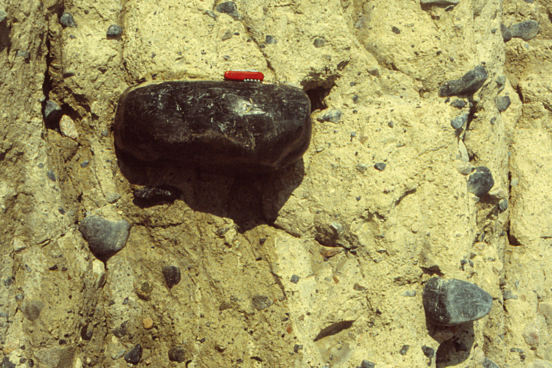
|

| Figure 7-3. Map of northern Great Plains showing Wisconsin (gray) and Independence (pre-Illinoian) glacial features. Location of Independence Formation stratotype is indicated by asterisk. Adapted from Aber (1991). |
The Independence glaciation likewise consisted of two ice lobes—Minnesota to the east and Dakota to the west. These two lobes were confluent over the crest of the Coteau des Prairies, but maintained their separate identities southward to the ice margin. The Minnesota lobe advanced southward through Iowa, into Missouri, and entered Kansas from the northeast. Conversely, the Dakota lobe came from the Dakotas, across Nebraska, and moved into Kansas from the northwest. Evidences from glaciotectonic structures and glacial striations confirm these two directions of ice advance in northeastern Kansas (Dellwig and Baldwin 1965).
Deposits of both ice lobes are present at the Independence Formation stratotype, near Atchison, Kansas—see Fig. 7-4. The lower till is a gray, wood-bearing, compact till that exhibits a large diapir and thrust faults. The diapir and thrusts extend up into fine sand and silt beds that were deposited in an ice marginal lake. Recumbent, isoclinal folds near the top of this sand were created by the ice advance that laid down the overlying upper till.
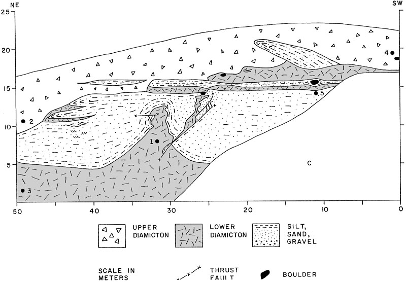
| Figure 7-4. Independence formation stratotype near Atchison, Kansas. Two tills separated by sand display a variety of ice-pushed structures. Section measured in m with no vertical exaggeration; taken from Aber (1985, fig. 4). |

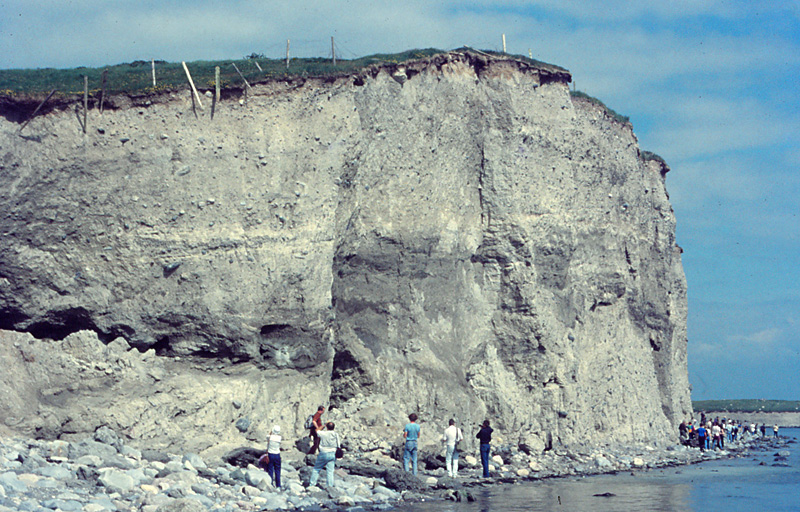
| Overview (left) of Independence Formation stratotype near Atchison, Kansas. Upper brown till (upper right) overlies deformed sand. Lower gray till (bottom left) is deformed in a diapir that intrudes sand in the middle of the section (behind ladder). Close-up view (right) of the large diapir of lower gray till. | 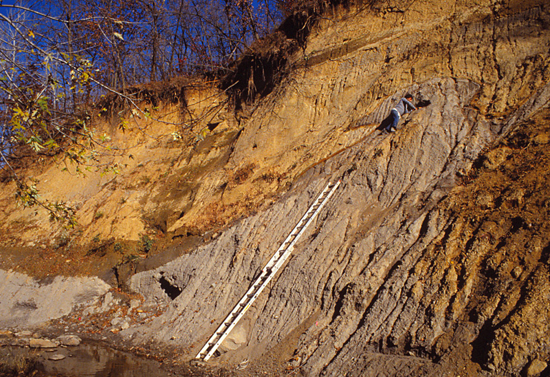 |

| Planed and striated limestone boulder embedded in lower gray till near site 3 (fig. 7-4). Knitting needle points in direction of ice movement from northeast to southwest. Silva compass for scale. |
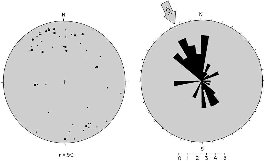
| Figure 7-5. Till fabric plots for upper Independence till (site 4, fig. 7-4). Rose diagram (right); equal-area stereonet (left). Total of 50 pebble long axes are plotted on each diagram. |
Tables 7-1 and 7-2 (below) present fabric data for sites 1 and 3 from the lower gray till in the Independence Formation stratotype (see fig. 7-4 for site locations). Forty-two measurements are given for site 1 and 50 for site 3. Use these data for the following.
| Trend/Plunge | Trend/Plunge | Trend/Plunge |
|---|---|---|
| 1. 250/40 | 15. 080/30 | 29. 157/27 |
| 2. 115/09 | 16. 295/32 | 30. 072/33 |
| 3. 077/00 | 17. 322/74 | 31. 220/06 |
| 4. 340/56 | 18. 295/15 | 32. 288/71 |
| 5. 335/57 | 19. 328/78 | 33. 130/46 |
| 6. 063/04 | 20. 000/90 | 34. 035/08 |
| 7. 317/36 | 21. 040/36 | 35. 270/25 |
| 8. 136/49 | 22. 298/21 | 36. 003/55 |
| 9. 015/60 | 23. 280/26 | 37. 336/24 |
| 10. 072/35 | 24. 042/70 | 38. 090/62 |
| 11. 034/61 | 25. 342/54 | 39. 257/26 |
| 12. 088/39 | 26. 048/25 | 40. 044/65 |
| 13. 135/07 | 27. 255/15 | 41. 078/34 |
| 14. 338/71 | 28. 070/56 | 42. 110/10 |
| Trend/Plunge | Trend/Plunge | Trend/Plunge |
|---|---|---|
| 1. 153/06 | 18. 071/30 | 35. 068/15 |
| 2. 153/12 | 19. 133/02 | 36. 082/26 |
| 3. 044/03 | 20. 112/23 | 37. 315/17 |
| 4. 130/08 | 21. 054/21 | 38. 053/15 |
| 5. 244/20 | 22. 074/27 | 39. 160/42 |
| 6. 085/35 | 23. 008/40 | 40. 136/19 |
| 7. 062/36 | 24. 086/01 | 41. 341/21 |
| 8. 138/20 | 25. 038/32 | 42. 150/24 |
| 9. 250/08 | 26. 009/47 | 43. 247/18 |
| 10. 272/00 | 27. 105/10 | 44. 250/11 |
| 11. 070/19 | 28. 145/25 | 45. 110/00 |
| 12. 036/20 | 29. 245/24 | 46. 070/04 |
| 13. 104/35 | 30. 082/25 | 47. 140/13 |
| 14. 186/08 | 31. 230/27 | 48. 028/25 |
| 15. 170/23 | 32. 270/15 | 49. 108/00 |
| 16. 298/30 | 33. 165/30 | 50. 080/14 |
| 17. 160/06 | 34. 110/32 |
To simplify plotting planes on the stereonet, it is convenient to plot the pole to each plane. The pole is a line running through the center of the projection sphere and perpendicular to the plane—see Fig. 8-1. The pole forms a 90° angle with the strike line and a 90° angle with the dip line. Thus, the pole is always be found in the opposite quadrant of the stereonet from the dip of the plane.
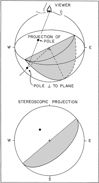
| Figure 8-1. Pole perpendicular to dipping plane in projection sphere (above), and the resulting stereographic projection of the plane and its pole (below). |
Figure 8-2 illustrates a surface folded in a cylindrical style around three parallel fold axes. Poles perpendicular to the folded surface are indicated in various positions. Note that all of the poles are perpendicular to the fold axes, regardless of their positions on the folded surface. In fact, the poles define a plane which is perpendicular to the fold axes.

| Figure 8-2. Poles on a series of northeast-plunging cylindrical folds (above), and the stereonet plot of those poles (below). On the stereonet, the poles fall on an arc that represents a plane perpendicular to the fold axis. |
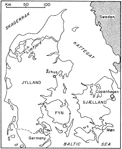
| Figure 8-3. Denmark location map. The Limfjord estuary extends across the northern part of the Jylland pennisula. Stipling shows crystalline bedrock in Sweden. |
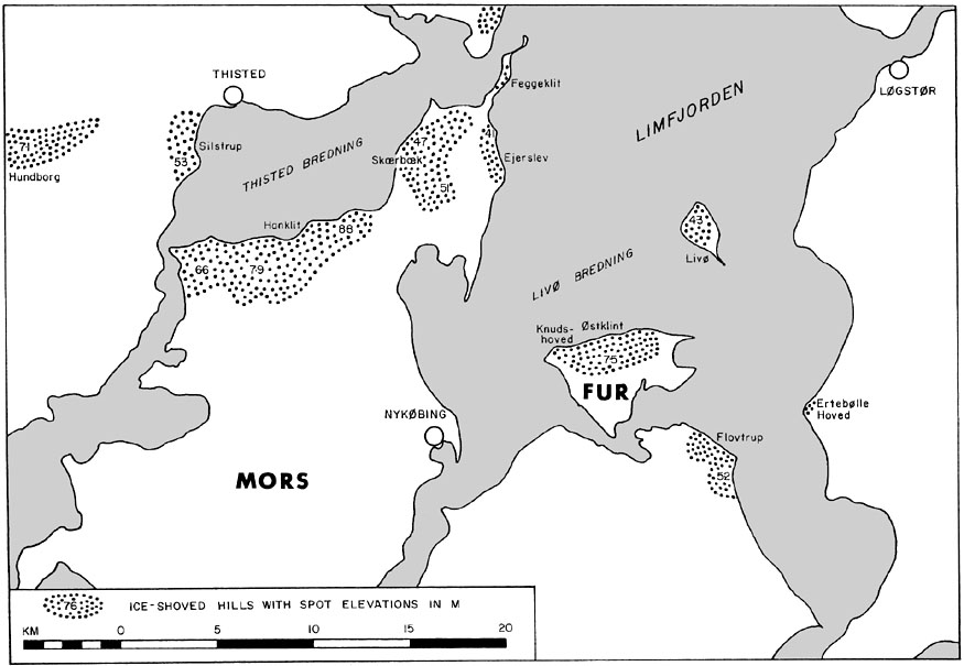
| Figure 8-4. Map of the Limfjord region of northern Jylland, Denmark showing zones of deformed Eocene strata (Fur Formation) in ice-pushed hills. The highest ridges exceed 70 m in elevation. Problem site is Ertebřlle Hoved on east side of map. |

| Large exposure of Fur Formation in Harhřj gravel pit on the island of Mors, Limfjord estuary, northwestern Denmark. Overturned syncline (left) with a core of glacial gravel leads into a sharply folded anticline (right) and another syncline. After folding, the structure was truncated by overriding ice. |  |
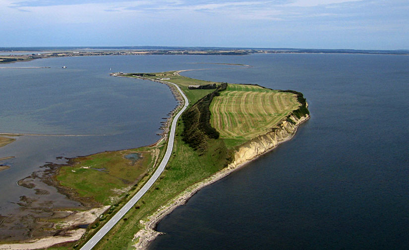
| Fegge, a peninsula at the northern end of the island of Mors in the Limfjord (see fig. 8-4). Kite aerial photo (left) and ground shot (right) showing the cliff exposure on the side of the flat-topped hill. The cliff reveals folded and thrust bodies of Fur Formation. | 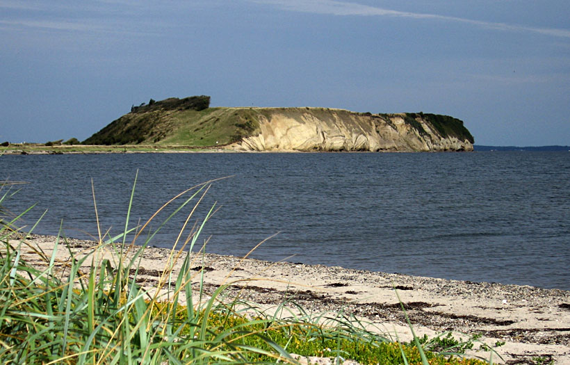
|
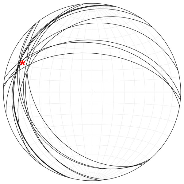
| Begin by entering the 14 strike-and-dip values for a planar dataset. The planes plot as arcs on the stereonet. Notice two sets of planes representing two fold limbs. You may visually approximate the fold axis at the point where most of the planes intersect (red asterisk). |

| Next convert the strike-and-dip values in Table 8-1 into pole values. Strike - 90 = pole trend; 90 - dip = pole plunge. For example, site 1: 279 - 90 = 189 (trend) and 90 - 44 = 46 (plunge). Enter the pole values in a new linear dataset. You should get a plot with 14 points that represent poles to planes. |
| Site | Strike/Dip | Site | Strike/Dip | ||||||||||||||||||||||||
|---|---|---|---|---|---|---|---|---|---|---|---|---|---|---|---|---|---|---|---|---|---|---|---|---|---|---|---|
Strike and dip according to the right-hand rule.
Adapted from Gry (1940, p. 588).
A stress unit commonly used in structural geology is the
kilobar (kb), which is 1000 bars or approximately 1000 atmospheres. For continental rocks of medium density, a pressure of 1 kb is achieved at a depth of 3˝ to 4 km (2 to 2˝ miles), and a pressure of 10 kb is reached at the base of continental crust. It was under such high-pressure conditions that plutonic and metamorphic
rocks now exposed in mountain belts and shields were created.
The high pressure imposed on deeply buried rocks due to
weight of the overburden is uniform and equal in all directions.
A similar, uniform pressure is experienced by underwater divers.
Such stress in crustal rocks is called lithostatic pressure, and it is determined solely by the thickness and density of the overburden. It is compressive or positive stress, in contrast to tension which is a negative stress.
Lithostatic pressure may produce strain in rocks due to
simple compaction, but it probably cannot account for most
folding and faulting. For this, differential stress is required.
Differential stress may be developed by unequal normal stresses
or by shear stress—see Figs. 9-1 and 9-2.
The standard means of portraying the behavior of a stressed
rock is with a stress-strain diagram, where strain is plotted on
the horizontal axis and stress is plotted on the vertical axis—see
Fig. 9-3. Strain is the percentage of shortening parallel to
õ1 and stress is the difference õ1 - õ3. As differential stress
increases, most rocks initially behave in an elastic manner. In other words, strain is directly proportional to stress, and strain disappears when stress is removed. This results in a straight line on the graph.
In order to drag the brick, a horizontal shear stress must
be applied. The total stress operating on the brick is the shear
stress plus the normal stress of gravity, and the total stress
vector forms an angle (ø) with the vertical. This represents the
angle of internal friction; its magnitude is a measure of frictional resistance to sliding of the brick. Now, suppose the brick is bonded to the underlying surface by mortar. An additional shear stress must be applied to break the bond before any movement could take place. This additional shear stress, labelled To, is the cohesive strength of the mortar.
A series of stress circles representing different test conditions for a particular rock may be plotted together to produce a Mohr failure envelope—see Fig.9-7. Each Mohr circle represents the õ1 and Ð conditions of shear fracturing for a given confining pressure (õ3). As confining pressure increases, the õ1 stress and Ð angle at which failure occurs also increase. The points of rock failure on each circle define a line that is more-or-less straight at lower confining pressures and flattens out toward higher confining pressures. This line is the failure envelope; its intercept with the shear-stress axis gives cohesive strength (To), and its slope is the angle of internal friction (ø). Any point on or above the failure envelope represents stress conditions that would cause the rock to fracture.
Based on Kulhawy (1975, table XI).
A temperate glacier, which is separated from its bed by a
film of meltwater, may develop basal shear stress up to 1 bar,
and basal shear stress may reach 10 bars for glaciers frozen to
the substratum (Weertman 1961). The lithostatic pressure developed at the base of a glacier is given by:
9. ROCK STRENGTH
Stress and strain
Geologic bodies may be deformed by application of stress or
pressure, and the resulting change in size or shape of the body
is called strain. Stress is simply force per unit area, and may
be expressed in such common units as: pounds per square inch
(psi), kg/cm², or atmospheres (1 atm. = 14.7 psi or about 1
kg/cm²) pressure.
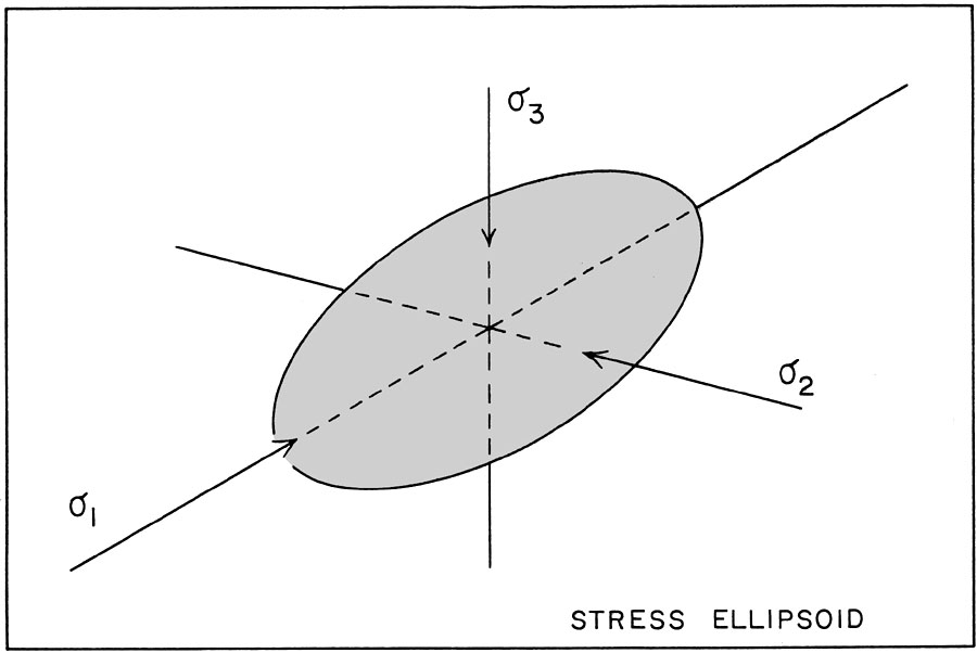
Figure 9-1. The stress ellipsoid: three normal (perpendicular) stress axes define the total stress applied to a rock body. õ1 is the maximum compressive stress, õ2 is the intermediate, and õ3 is the minimum. Normally, all three stresses are compressive; however, õ3 may be negative (tensional) in some cases. Where only lithostatic pressure is developed, the stresses are equal and the stress ellipsoid becomes a sphere.
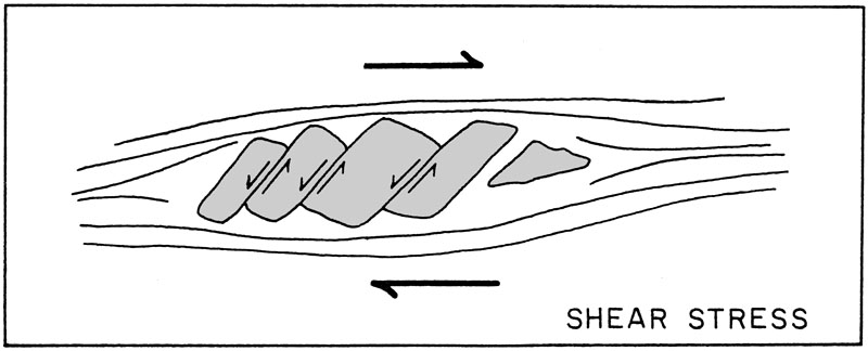
Figure 9-2. Hard augen, such as feldspar, within a ductile schist subjected to shear stress parallel to foliation. The sense of shear on oblique microfractures of augen is opposite to overall sense of shear in the rock. T symbolizes shear stress. Adapted from Simpson and Schmid (1983, fig. 9).
           change in length
     e  =  ---------------- x 100, where e = percent strain.
           original length
The amount of strain is, of course, related to the magnitude
of stress, and the strain response of various rocks to stress may
be tested in laboratory apparatus. Prepared rock cores are
squeezed in a hydraulic press subjecting the rock to high õ1
compression. Measuring devices attached to the press and rock sample monitor pressure and detect minute strains in the rock. Pressures as high as 100 kb could be produced by uniaxial or triaxial hydraulic presses. The highest experimental compression yet achieved is produced by a diamond-anvil technique that has reached pressures of 1700 kb (Jayaraman 1984).
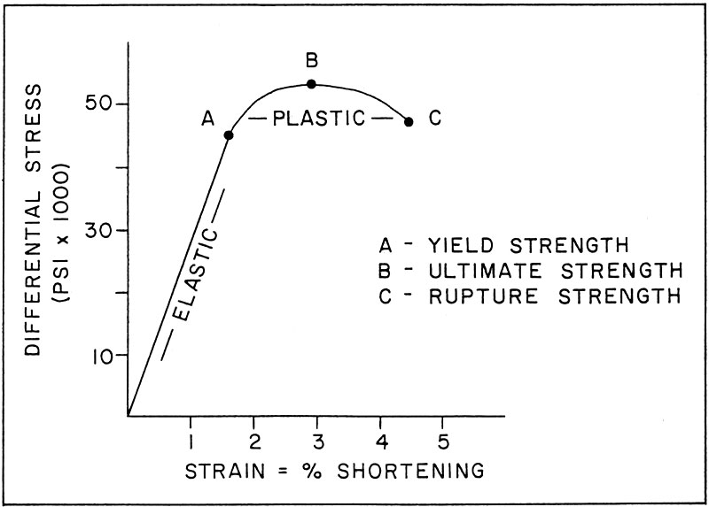
Figure 9-3. Typical stress-strain diagram showing the behavior of a limestone subjected to increasing õ1 stress under a high confining pressure. Adapted from Davis (1984, fig. 5.25).
Rock failure
The failure of a rock by rupturing results in characteristic sets of fractures whose orientations are related to the õ1, õ2, and õ3 stress axes—see Fig. 9-4.

Figure 9-4. Fractures produced experimentally in a block of Solenhofen limestone under differential stress. Fracture sets A and B are conjugate shear fractures, C are extension fractures, and D are release fractures. Adapted from Hobbs et al. (1976, fig. 7.31).
Shear fractures are the most common type of geologic fracture, and they develop because of the stress difference between õ1 and õ3. As õ2 is an intermediate stress, it may be ignored and shear fracturing analyzed in two dimensions—see Fig. 9-5A. Consider a plane within the rock which forms an angle (Ð) with the õ1 axis. The õ1 stress operating on the plane is composed of two components: (1) n1, a normal stress at right-angle to the plane, and (2) T1, a shear stress parallel to the plane. Likewise, the normal and shear stress components of õ3 may be determined and added to n1 and T1 to give the total normal stress (nt) and shear stress (Tt) operating on the plane. It is possible to calculate the total normal and shear stresses for a plane of any orientation using the following formulas.
           õ1 + õ3     õ1 - õ3
     n  =  -------  -  ------- (cos 2Ð)
              2           2

           õ1 - õ3
     T  =  ------- (sin 2Ð)
              2
Where õ1 > õ3, shear stress is developed on all planes except those oriented Ð = 0° or 90°, and maximum shear stress is achieved on the plane at Ð = 45°. As rock shear strength is generally much less than compressive strength, shear fractures tend to develop obliquely to the õ1 axis during differential compression.
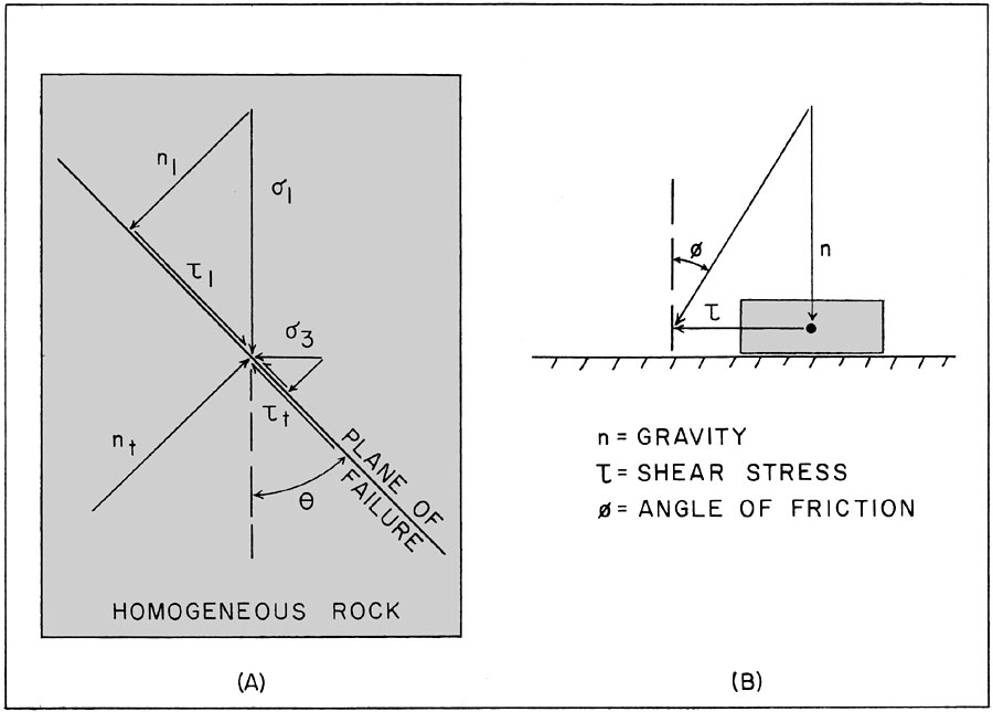
Figure 9-5. A - components of normal (n) and shear (T) stresses affecting a plane of potential failure within a rock. Ð is the angle between the maximum stress and the plane of failure. B - normal stress (gravity), shear stress (T), and angle of friction (ř) for a brick being dragged over a horizontal surface.
Mohr diagram
The Mohr stress circle provides a convenient graphical
means of solving the normal and shear stress equations presented
in the previous section. Normal stresses are plotted on the
horizontal axis and shear stress read on the vertical axis—see Fig.
9-6. A semicircle with its center on the normal stress axis at
(õ1 + õ3)/2 connects õ1 and õ3, and the radius of the semicircle equals (õ1 - õ3)/2. The angle 2Ð is measured from õ3 in clockwise direction.
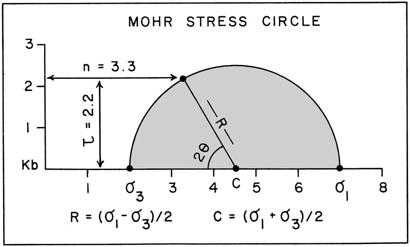
Figure 9-6. Basic Mohr diagram showing normal stress (horizontal axis) and shear stress (vertical axis) developed on a plane at Ð = 30° (2Ð = 60°) with ő1 = 7 kb and ő3 = 2 kb. Solving the stress equations for this situation gives n = 3.25 kb and T = 2.17 kb.
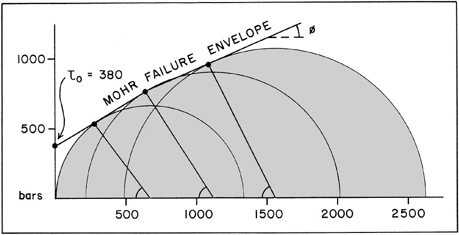
Figure 9-7. Mohr failure envelope for Carrara Marble. To represents cohesive strength, and ř is the angle of internal friction.
As many rocks possess an internal angle of friction of
approximately 30°, the Ð angle of shear fractures is
typically also about 30°.
Rock Type ř To
Igneous: Plutonic 45.6 561
Igneous: Volcanic 24.7 322
Metamorphic: Foliated 27.3 457
Metamorphic: Non-foliated 36.6 229
Sedimentary: Clastic 29.2 317
Sedimentary: Chemical 35.9 263
All Types (average) 32.0 345
Problem
Andrews (1980) has described glacial thrusting of Paleozoic limestone and shale along Densmore Creek in western New York near Rochester—see Fig. 9-8. A bedrock mass consisting of limestone and weathered shale has been thrust along a zone of brecciated shale containing disoriented angular blocks of limestone—see Fig. 9-9. Below this thrust, till rests on intact Irondequoit Limestone at the western end of the section, and overturned folds are developed in the limestone at the eastern end of the section.
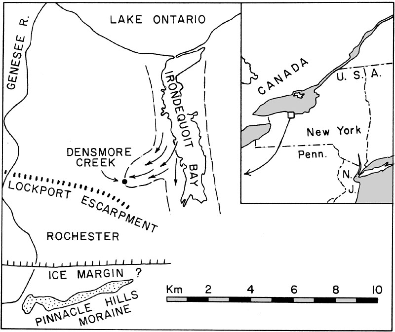
Figure 9-8. Map of Densmore Creek and vicinity showing local ice movement (arrows) along bedrock valley (dashed line) of Irondequoit Bay. Based on Andrews (1980, figs. 1 and 6).
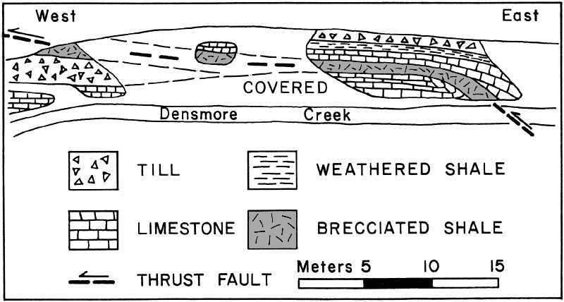
Figure 9-9. Densmore Creek section showing thrust bedrock mass. Thrust zone is located within a brecciated shale unit. Based on Andrews (1980, fig. 2).
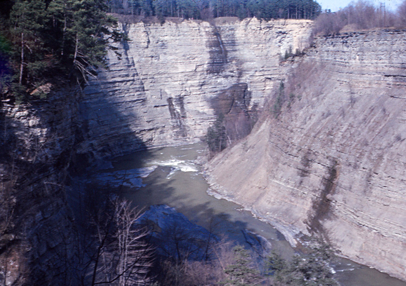
Genesse River gorge in western New York, near Rochester. Known as the Grand Canyon of the East, a thick sequence of upper Devonian clastic strata is exposed in the walls of the gorge.
References
![]() Return to Table of Contents.
Return to Table of Contents.