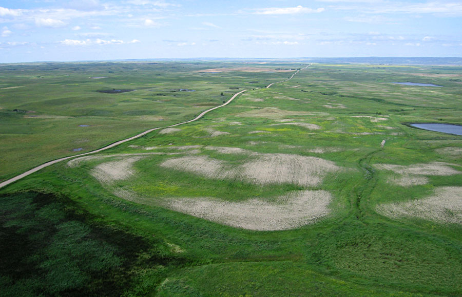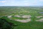
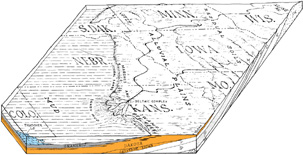
| Figure 1-6. Northern Dirt Hills, Saskatchewan, Canada. One of the largest ice-shoved-ridge complexes in the world. Notice the wavy road that passes over a series of ridges. Each ridge is underlain by an upthrust block of Cretaceous bedrock and covered by a thin veneer of glacial sediment. At least 200 m of vertical bedrock uplift are documented in the Dirt Hills (Aber and Ber 2007). Kite aerial photograph looking westward.
|
Organization of exercises
Most exercises in this lab manual involve actual geological
examples from North America and northern Europe. This case-history approach seems preferable to made-up exercises that may bear little relationship to real geology. Because of the use of actual situations, some exercises do not have a single right solution. Multiple correct answers are possible in some cases, and the
student would have to use some judgement in selecting the most
reasonable possibility given the data at hand. Far from being a
drawback, this is a more realistic representation of the daily
work of structural geologists.
Several of the exercises are amenable to computer analysis with various software programs. If the necessary software and hardware are available, students are encouraged to work through exercises using both
traditional graphical techniques and computer analysis. Metric
and English units are both used in this lab manual, and students
should become familiar with conversion between the two.
The following materials or equipment are necessary to complete all the lab exercises for this course. Each student should provide the following.
- Pencils - hard drafting pencils and colored pencils (or pens).
- Ruler - measured in cm/mm or tenths of inches.
- Protractor - measured in degrees.
- Compass - drafting bow or circle templates.
- Graph paper - measured in cm/mm or tenths of inches.
- Tracing paper - flat pad (not rolled).
- Tape - masking tape is preferable kind.
- Calculator - scientific style with trig and inverse trig functions.
- Stereonet 11 shareware for rose diagrams, stereographic projections, etc.
References
- Aber, J.S. 1988. Structural geology exercises with glaciotectonic examples. Hunter Textbooks, Winston-Salem, North Carolina, 140 p.
- Aber, J.S. and Ber, A. 2007. Glaciotectonism. Developments in Quaternary Science 6, Elservier, Amsterdam, 246 p.
- Aber, J.S., Croot, D.G. and Fenton, M.M. 1989. Glaciotectonic landforms and structures. Kluwer, Dordrecht, the Netherlands, 200 p.
- Berthelsen, A. 1979. Recumbent folds and boudinage structures formed by sub-glacial shear: an example of gravity tectonics. In, van der Linden, W.J.M. (ed.), Van Bemmelen and his search for harmony. Geologie en Mijnbouw 58, p. 253-260.
- Pedersen, S.A.S. 2005. Structural analysis of the Rubjerg Knude glaciotectonic complex, Vendsyssel, northern Denmark. Geological Survey of Denmark and Greenland, Bulletin 8. Access online.
- Sauer, E.K. 1978. The engineering significance of glacier ice-thrusting. Canadian Geotechnical Journal 15, p. 457-472.
2. PLANAR STRATA
Geometric elements in structural geology
Geologists must deal with structures developed on all scales
from microscopic to continental within all manner of materials
from loose sediments to high-grade metamorphic complexes. Some
of these structures are geometrically simple, but many are
irregular and complex in form due to multiple phases of
deformation. All structures, regardless of their complexity, may
be reduced to combinations of two basic geometric elementsóplanes and lines, the orientations of which may be determined.
Planar features within rocks include bedding planes and planar cross beds; crystal faces; joints, faults, dikes, fissures and other fractures; veins, foliation, schistosity, cleavage and partings; fold axial planes; seismic discontinuities; water table; formation and other stratigraphic boundaries; and unconformities.
Linear features within rocks include striations, grooves, troughs and channels; yardangs; axes of pebbles, shells, augens, and of other elongated objects; crests of ripples, dunes, drumlins, and of other elongated sedimentary forms; crystallographic and optic axes of minerals; lineations; intersections of fractures or other planar features; fold axes; paleomagnetic axes; rotation axes of plates; strike and dip lines; and lineaments.
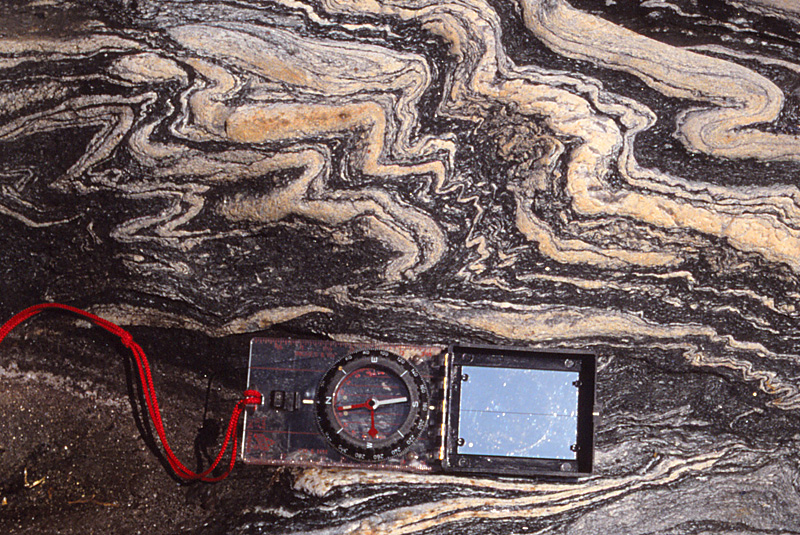
 Geometric elements of structural geology.
Orientations of planes and lines
The orientation of a plane relative to the Earth's surface is determined by two measurements, namely strike and dip. Strike is defined as the compass direction of a horizontal line in the
plane. Compass directions are customarily measured in degrees
from 0 to 360∞, or could be recorded as N50E, N45W, S15E, etc. Dip
is the direction and angle of maximum downward tilting, which is
always perpendicular (90∞) to strike.
The house roof shown in Figure 2-1 illustrates strike and dip in a tilted plane. The horizontal crest of the roof represents the strike with a compass direction of 50∞ (or N50E). The dip direction of the roof is SE, perpendicular to the strike: 50 + 90 = 140∞ (or S40E), and the dip angle measured from horizontal is 30∞.
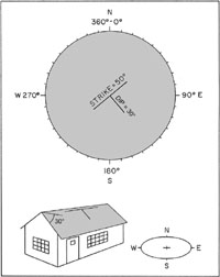
| Figure 2-1. Schematic diagram of a house roof (below) with
a strike-and-dip symbol and compass diagram (above).
|
Measurements are always made relative to true north rather
than magnetic north. The most common compasses carried by field
geologists are the Brunton Pocket Transit or the Silva Ranger. Both include built-in mechanisms for making magnetic declination adjustments and levels for measuring dip angles. With one of these relatively simple instruments, the field geologist may collect a great deal of information concerning the planar and linear elements for all kinds of structures.
The "T" symbol shown on Figure 2-1 is used to indicate
strike-and-dip measurements on maps and diagrams. The long
cross-line represents strike, and the shorter stem represents the
dip direction. The dip angle is sometimes given next to the dip
line. Variations of the basic strike-and-dip symbol are used for
different planar featuresósee Fig. 2-2.
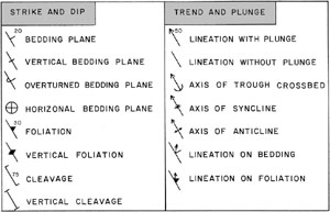
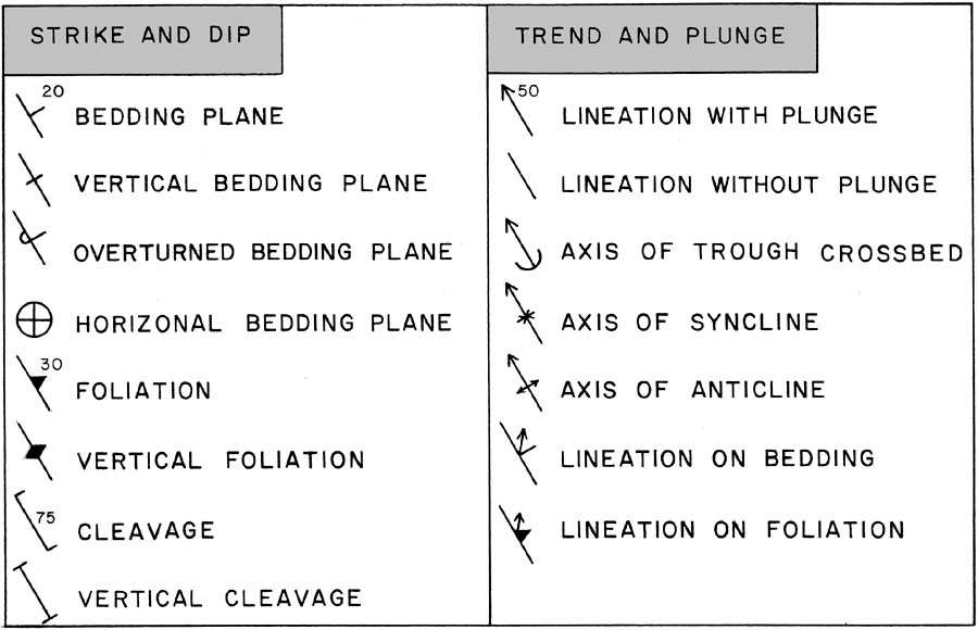
| Figure 2-2. Geologic symbols for planar
features (left) and linear features (right).
|
The orientation of a line relative to the Earth's surface is likewise determined by two measurements, namely trend and plunge. Trend is defined as the compass direction of the line, and plunge is
the direction and angle of downward tilting of the line. In
Figure 2-1, the strike line has a trend of 50∞ and a
plunge of 0∞. The dip line has a trend of 140∞ and
a plunge of 30∞. The basic map symbol for a linear
measurement is simply a short line with or without an arrow at
one end to indicate the direction of plunge (fig. 2-2). A word
of caution: trend and plunge refer to linear features, whereas
strike and dip refer to planar featuresódo not confuse them.
Finding the orientation of a plane
Geometrically, any three points, which are not in the same
line, define a plane. Given a recognizible planar feature, such
as a marker bed or mineral vein, the strike and dip of that
planar feature could be determined if its elevation is known at
three points. The elevation control points may be in either surface or subsurface locations.
One common situation involves three nearby wells drilled
into the same tilted horizon. The orientation of that horizon
may be easily calculated and projected into the surrounding area.
The same procedure could also be applied to surface outcrops or to
a combination of surface and subsurface control points. Note
that deep subsurface elevations are often below sea level, and so
are negative.
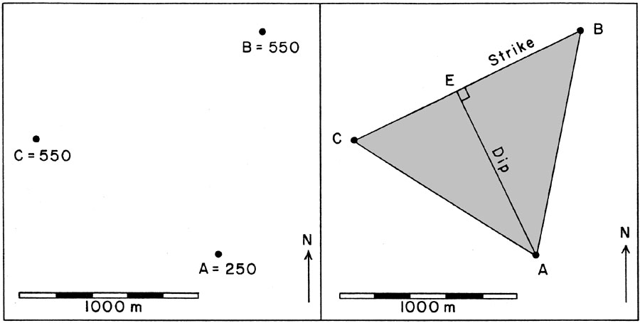
Figure 2-3 shows a map view of three points for which the
elevations of a distinctive bed are known. The three points are
labelled as follows: A = low point, B = intermediate point, and
C = high point. In this special case, B and C are equal in
elevation. To find the strike and dip, first connect the three
points with straight lines forming a triangle.

| Figure 2-3. Map of sample three-point problem.
Elevations are given for a unique planar feature
(left). Solution for strike and dip shown on right.
|
This planar triangle represents the dipping bed. Recall
that strike is a horizontal line in the plane, that is a line of
equal elevation; thus line CB is the strike. Its compass
direction may be measured off the map. Next, draw a line which
is perpendicular to the strike line CB and which passes through
point A, the low point. This is the dip line (AE) and its
compass direction equals strike direction plus 90∞. The dip angle is given by a simple expression:
(elevation E - elevation A) ˜ (map distance AE) = tan (dip angle).
In this case, 300 ˜ 1020 = tan 16∞. So, strike = 64∞ and dip = 16∞. This example was easy to work with because two points are at the same elevation and, thus, automatically define the strike line.
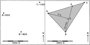
| Figure 2-4. Map of sample three-point problem.
Elevations are given for a unique planar feature
(left). Solution for strike and dip shown on right.
|
In the more general case, as illustrated in Figure 2-4, all
three points have different elevations. Again, the points are
connected to form a triangle and labelled with A lowest, B
intermediate, and C highest. Point B serves as one end of
the strike line; the other end is point D located somewhere
along line AC. The exact location of point D is found by a
ratio of distances to elevations:
(elevation B - elevation A) ˜ (elevation C - elevation A) = distance AD ˜ distance AC
Point D found in this manner is equal in elevation to point
B; thus line BD is the strike. Next draw the line AE, which is
perpendicular to line BD, and continue with the same steps as
before to find the dip. In Figure 2-4, distance AD = 1000 m,
strike = 195∞, and dip = 25∞. Practice this calculation to gain experience with solving three-point problems.
Apparent dip and true dip
The true or maximum dip angle is measured only perpendicular to the strike line, as shown by the house roof (Fig. 2-1). A dip angle measured in any other direction would be less than true dip and is called apparent dip.
Consider, for example, a vertical, E-W cross section through
the house of Figure 2-1. The section cuts diagonally across
the roof, which appears to dip in the section at an angle
less than 30∞. Another cross section running parallel to
strike (50∞) would show no dip; the roof would appear horizontal. The relationship between true dip and apparent dip is defined by the following functions:
- tan AD = tan TD x cos A, or
- tan AD = tan TD x sin B,
where:
- TD = true dip angle.
- AD = apparent dip angle.
- A = compass angle between true dip and apparent dip trends.
- B = compass angle between apparent dip trend and strike.
Note: apparent dip is always less than true dip, which is the maximum dip possible on a tilted plane.
Problem
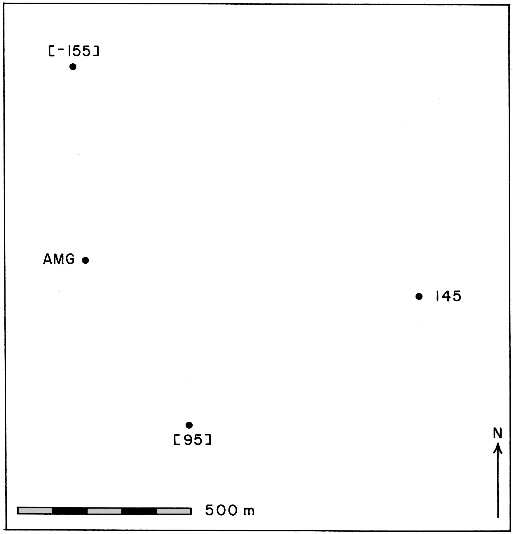
The large-scale map shows three control points on a distinctive mineralized vein, which outcrops in a roadcut at the eastern point and has been encountered below hills in drill holes to the westósee Fig. 2-5. The vein is assumed to be planar and is of considerable economic interest, as it is known locally to contain malachite, an indicator for possible gold or other valuable metals.
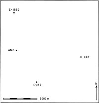
| Figure 2-5. Map of three-point problem. Elevations in [ ] are subsurface; note one elevation is below sea level. AMG = Amerigold mine site. Print the map at full size, and complete this problem following the examples given above.
|
- Determine the strike and dip of the mineralized vein.
- The ficticious "Amerigold Company" owns a mining lease at
the point labelled AMG. If this site has a land elevation
of 158 m, how deep would the miners have to dig in order
to reach the mineralized vein at that point? Hint: construct a dip line from AMG to your strike line.
3. PRIMARY STRUCTURE
Introduction
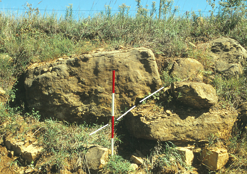
Primary structures are those features created in a rock at the time of its original deposition (sedimentary), cooling (metamorphic), or solidification from magma or lava (igneous). Such features are part of the rock body from its genesis. Recognition of primary structures is important to distinguish from later structures caused by stress, strain, and the resulting deformation of the rock body.
Primary structures.
Problem
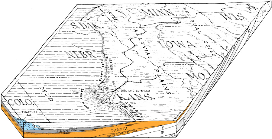
The Dakota Formation of middle Cretaceous age in north-central Kansas is famous for its cross bedding. The Dakota was deposited in various coastal, deltaic, and shallow marine environmentsósee Fig. 3-1.
| Figure 3-1. Reconstruction of Cretaceous strata and environments of Kansas at the time of Graneros marine transgression over coastal, deltaic, and alluvial plain deposits of the Dakota Formation. Adapted from Hattin and Siemers (1978 fig. 3).
|
Cross-bedded sandstones fill large channels within finer siltstone and shale. The cross bedding consists of small- and
medium-scale, planar or lenticular sets. The planar style with high angle of dip (>20∞) is most common (Franks et al. 1959). Such cross bedding is particularly well displayed where it crops out in large concretions, as at Rock City near Minneapolis in Ottawa County, Kansas.
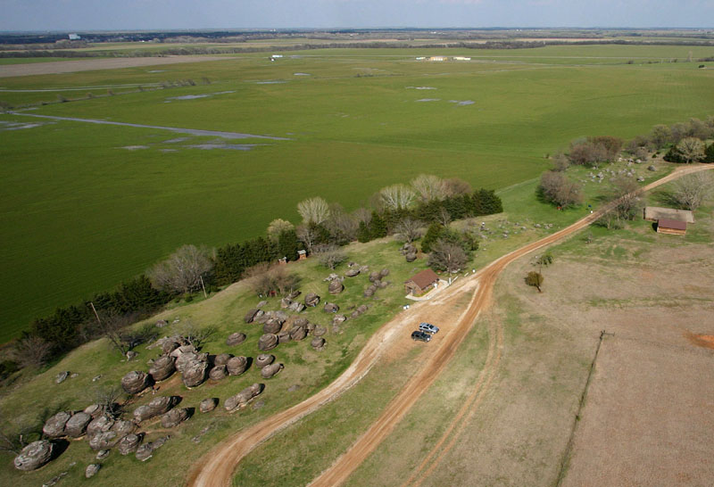
 Rock City, Minneapolis, Kansas
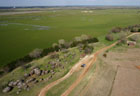
| Aerial overview of large concretions exposed along the bluff next to the Solomon River valley. Grain elevator at Minneapolis appears in the left background. Helium-blimp airphotos. |
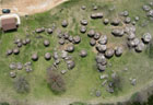
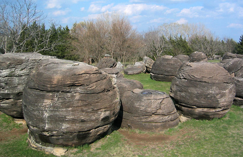
| Close-up vertical shot of large concretions. Most are nearly spherical and appear like giant bowling balls. Some are joined into double or triple spheres. The single spheres are 15-25 feet (5-8 m) in diameter. |
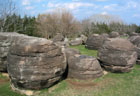
| Ground view of large sandstone concretions. Note distinctive cross bedding displayed by these concretions. Images adapted from Aber and Aber (2009). |
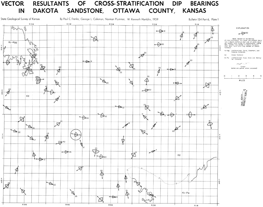
Detailed investigation of sandstone cross bedding was undertaken in Ottawa County by
Franks et al. (1959), who constructed the accompanying mapósee Fig. 3-2. The map shows average cross
bed directions (vectors) for 79 sites, the number of measurements at each site, and the
standard deviation of measurements at each site.
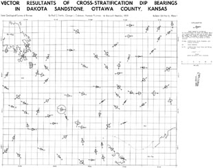
| Figure 3-2. Map showing directions of cross-bedding (dip trends) for sandstone in the Dakota Formation of Ottawa County, north-central Kansas. Notice the diversity of results. Taken from Franks et al. (1959).
|
A table of data for each site is also includedósee Table 3-1. For this lab, you will make a rose (compass) diagram of the data and interpret the depositional environment from the rose diagram, map, and other information.
Table 3-1. Cross-bedding vector data in azimuth degrees. Adapted from Franks et al. (1959, Table 1).
| 1. 82 | 2. 54 | 3. 53 | 4. 54 |
| 5. 70 | 6. 95 | 7. 142 | 8. 113 |
| 9. 174 | 10. 92 | 11. 169 | 12. 175 |
| 13. 164 | 14. 117 | 15. 133 | 16. 131 |
| 17. 137 | 18. 167 | 19. 136 | 20. 149 |
| 21. 175 | 22. 174 | 23. 121 | 24. 233 |
| 25. 236 | 26. 216 | 27. 233 | 28. 222 |
| 29. 212 | 30. 219 | 31. 202 | 32. 265 |
| 33. 203 | 34. 204 | 35. 199 | 36. 270 |
| 37. 206 | 38. 221 | 39. 230 | 40. 239 |
| 41. 231 | 42. 236 | 43. 268 | 44. 186 |
| 45. 192 | 46. 205 | 47. 235 | 48. 260 |
| 49. 199 | 50. 252 | 51. 215 | 52. 267 |
| 53. 210 | 54. 290 | 55. 294 | 56. 297 |
| 57. 284 | 58. 315 | 59. 274 | 60. 273 |
| 61. 274 | 62. 280 | 63. 291 | 64. 326 |
| 65. 340 | 66. 306 | 67. 270 | 68. 275 |
| 69. 290 | 70. 305 | 71. 320 | 72. 325 |
| 73. 298 | 74. 321 | 75. 282 | 76. 305 |
| 77. 282 | 78. 279 | 79. 316 |
Lab procedures
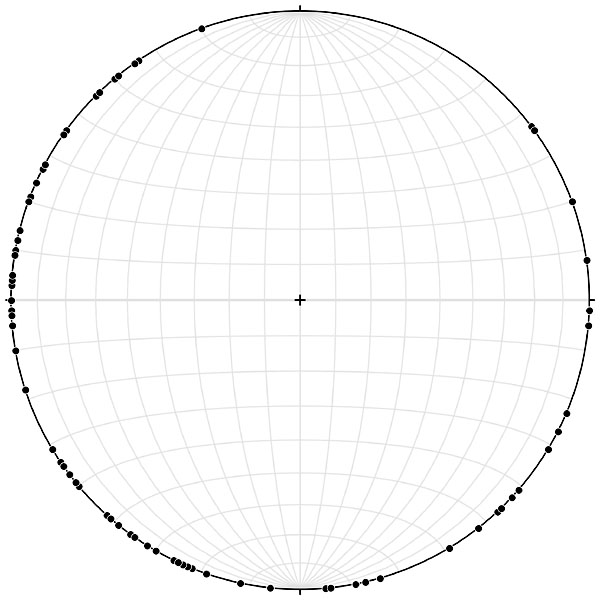
- Use Stereonet 11 shareware to create the necessary file. Make a linear dataset. Enter each azimuth value in the trend column. Note: plunge values = zero for all entries. Save your file periodically as you enter values.
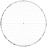
| Your data file should have 79 trend/plunge values, which appear as 79 points on the outer perimeter of the stereonet display. However, some of the dots overlap and may be difficult to see individually, so visual inspection is difficult. |
- Next create a rose diagram. This display resembles a circular bar graph that should aid your visual interpretation of the cross-bedding pattern.
- Interpret the regional pattern of paleocurrents as displayed on the rose diagram
and the map (above). Briefly describe the likely depositional environment and paleogeography
for the Dakota Formation. The paleocurrent patterns of some common sedimentary
environments are given belowósee Table 3-2.
 Table 3-2. Paleocurrent patterns of deposition.
Environment | Local current vector | Regional pattern |
| Alluvial, braided | unimodal, low variability | diverging |
| Alluvial, meandering | unimodal, high variability | converging |
| Delta | unimodal, high variability | radiating |
| Aeolian | uni-, bi-, or polymodal | large arc |
| Shore line/shelf | bimodal (tides) or other | 90∞ or parallel
to coast line |
| Continenal slope | unimodal (turbidites) | radiating |
References
- Aber, J.S. and Aber, S.W. 2009. Kansas physiographic provinces: Bird's-eye views. Kansas Geological Survey, Educational Series 17, 76 p. Go to KGS.
- Franks, P.C., Coleman, G.L., Plummer, N. and Hamblin, W.K. 1959. Vector resultants of cross-stratification dip bearings in Dakota Sandstone, Ottawa County, Kansas. Kansas Geological Survey, Bulletin 134, part 6, plate 1.
- Hattin, D.E. and Siemers, C.T. 1978. Upper Cretaceous stratigraphy and depositional environments of western Kansas. Kansas Geological Survey, Guidebook Series 3.

 Return to Table of Contents.
Notice: This course was prepared for the use and benefit of students enrolled at Emporia State University. Others are welcome to view the course webpages. Any other use of text, imagery or curriculum materials is prohibited without permission. © J.S. Aber (2021).