| with Glaciotectonic Examples
James S. Aber, Professor Emeritus
Exercise Solutions |
|
| with Glaciotectonic Examples
James S. Aber, Professor Emeritus
Exercise Solutions |
	elevation B - elevation A     250   distance AD     AD
	-------------------------  =  --- = -----------  = ----
	elevation C - elevation A     300   distance AC    1200
AD = 1000, and line BD is the strike = N45E (225°). Draw the dip line AE perpendicular to line BD. Calculate the dip angle:
	elevation E - elevation A     250
	-------------------------  =  ---  =  tan (dip angle).  Dip angle = 14° (NW).
	map distance AE               980
	elevation E (95) - elevation AMG
	--------------------------------  =  tan 14°
	map distance of dip line (550)
Elevation of AMG = -42 m. Subtract elevation of vein at AMG from land surface elevation to determine depth: 158 - (-42) = 200 m.
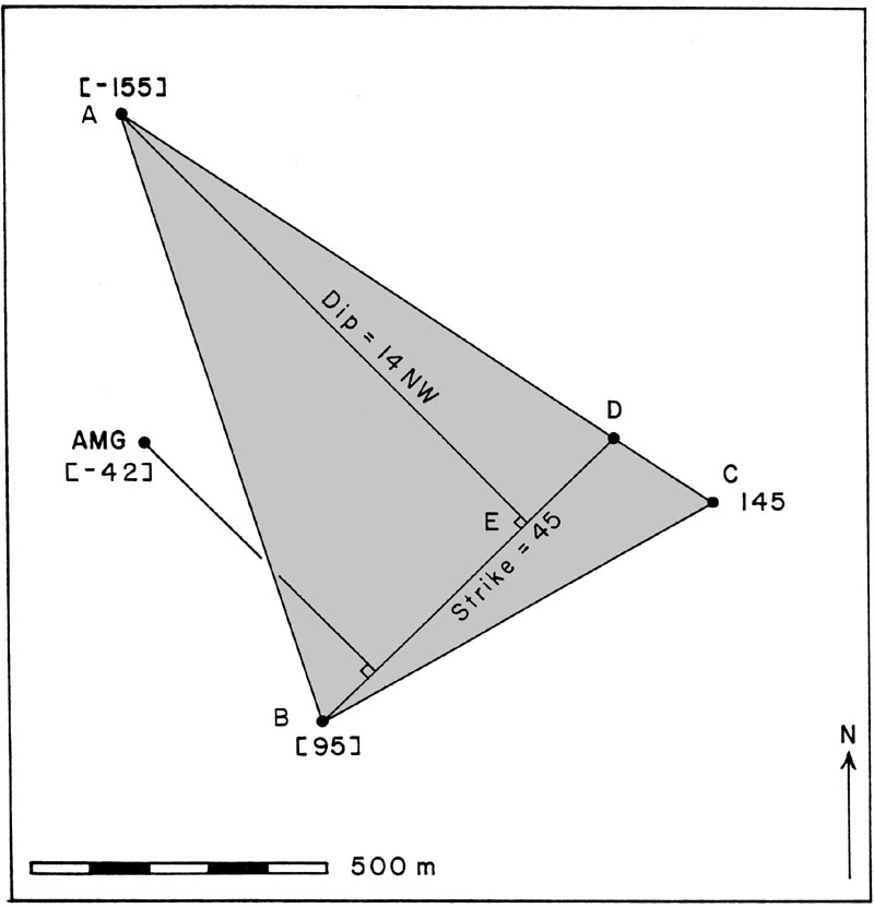
| Strike-and-dip triangle map |
The cross-bedding pattern is bimodal and/or multi-modal with a strong mode toward the southwest, a secondary mode to WNW, and several lesser modes in other directions. The regional pattern is likewise highly variable. This suggests multiple meandering channels on an alluvial plain and/or delta complex.
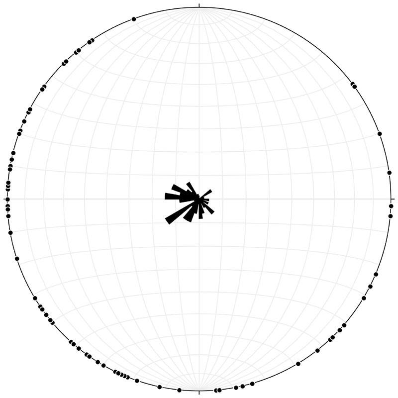
| Rose diagram for Dakota cross bedding |
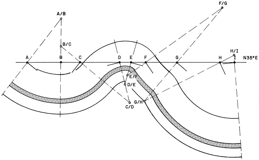
A = 38° NE, B = horizontal, C = 51° SW, D = 14° SW, E = 15° NE, F = 55° NE, G = 42° NE, H = 63° NE, and I = 5° SW.
 |
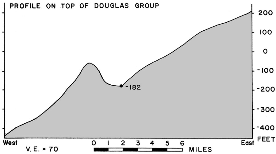
The vertical cross-section scale of 1 inch = 200 feet (2400 inches) is 1/2400 or 1:2400. The resulting vertical exaggeration equals 68,960/2400 or approximately 70 times.
The two points are approximately 24,640 feet apart and 205 feet different in elevation. Applying the dip-angle formula: 205/24,640 = tan (dip angle); dip angle = 0.5° W, or 44 feet per mile.
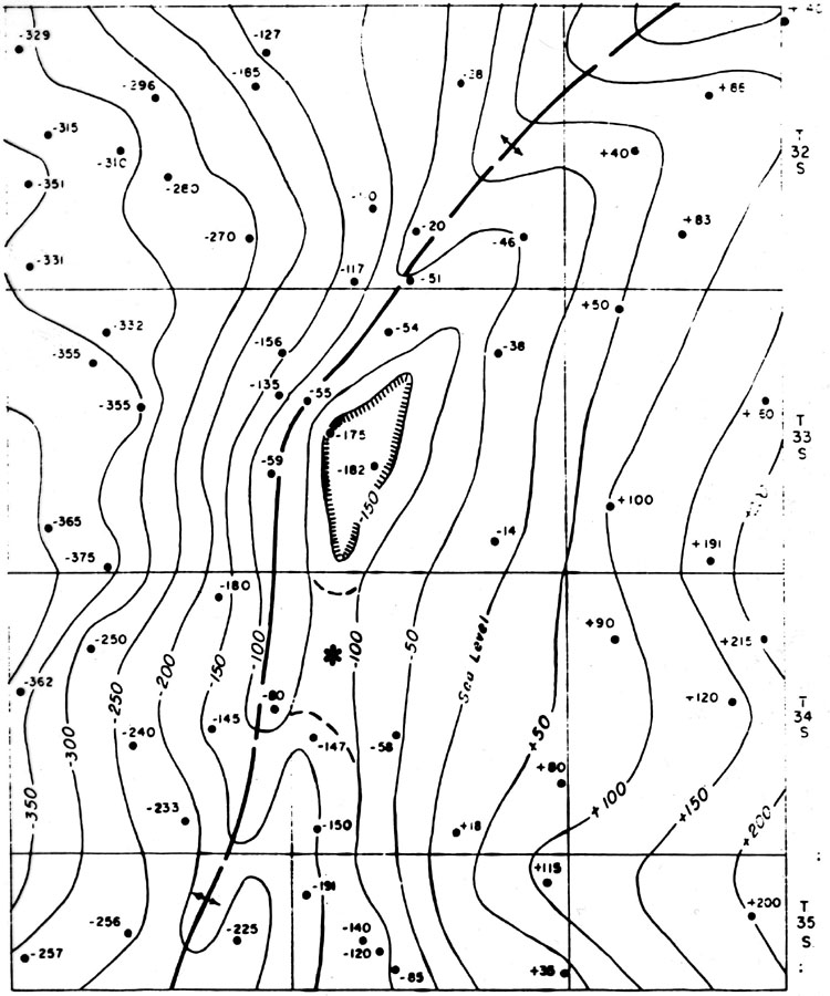
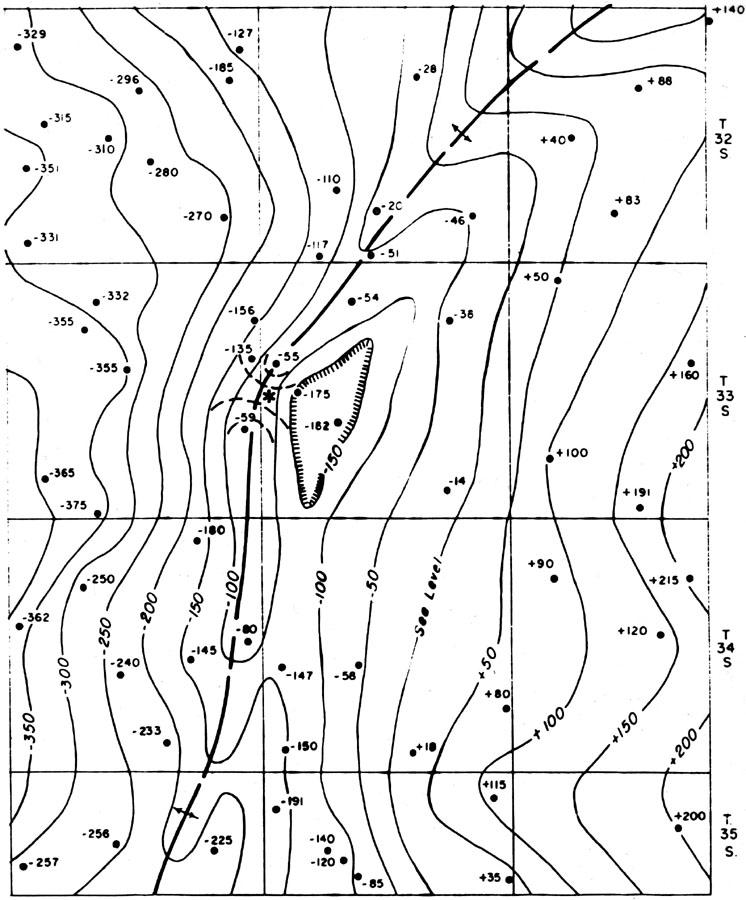
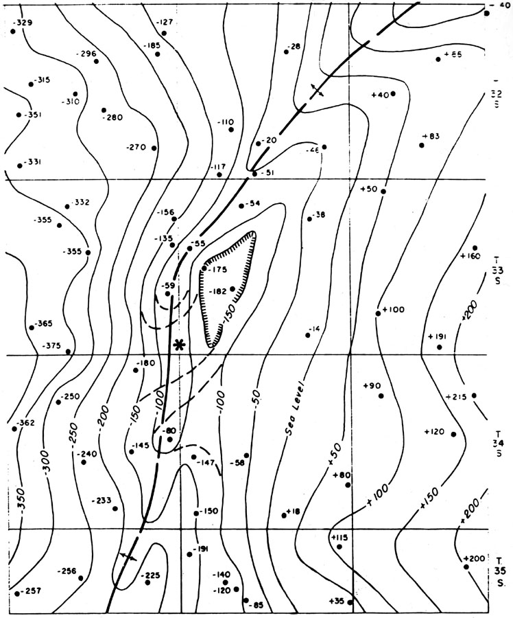
This variation is perhaps the simplest and the one that many students will give; it does not significantly alter the overall structural pattern, as an anticline is still evident immediately to the west. Bayne's map and this first variation are preferred, because they conform with the surface expression of the Dexter Anticline.
These variations do represent significantly different structural patterns, but they are equally correct based on the available subsurface data. Still other contour configur-ations and structures are possible in the central portion of the map area. The instructor should examine each version carefully to ascertain its correctness based on the data.
  |
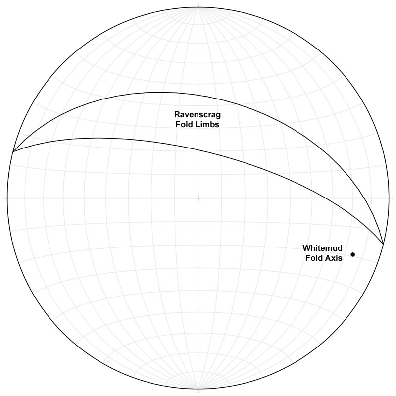
| Dirt Hills folds |

 |
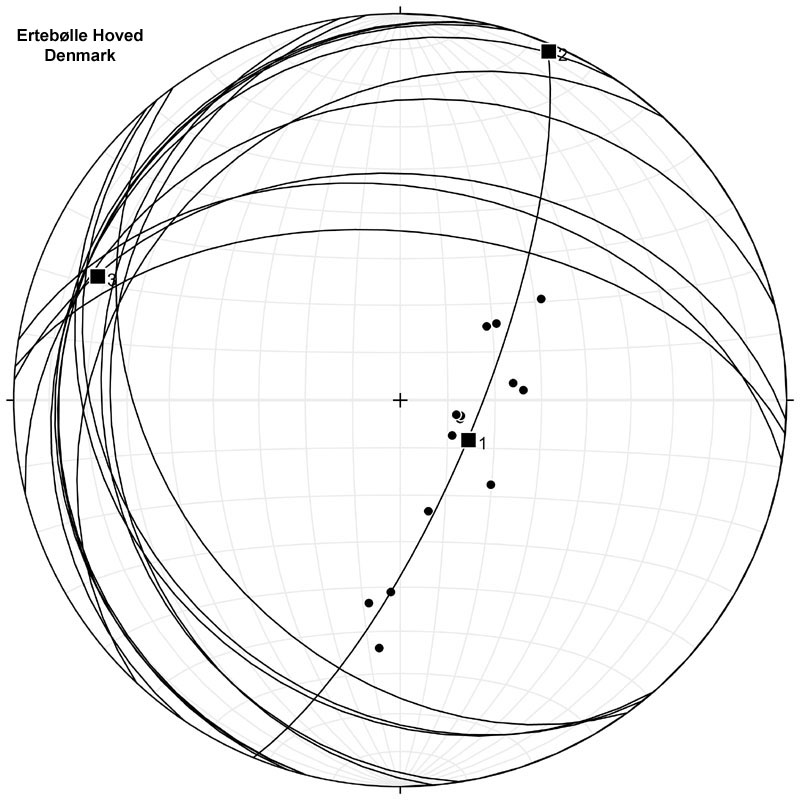
| Ertebřlle Hoved constructed fold |
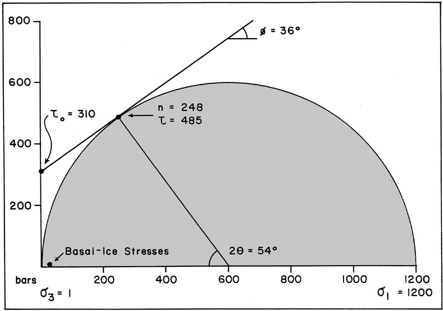 Mohr diagram – Irondequoit Limestone |
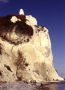
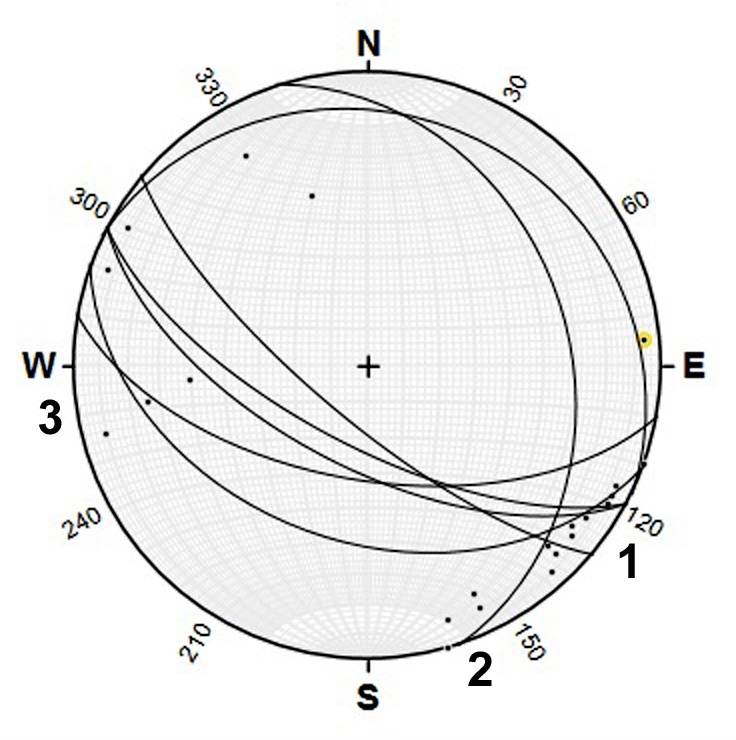 Folds and faults at Hvideklint, Hjelm Nakke, and Vagtbo Bakke. |
havD = (cos65 x cos62 x hav10) + hav(65 - 62). D = 5.4°.5.4° of a great circle = 5.4 x 111 km = 599.4 (app. 600) km. Average linear velocity equals length divided by time:
	V  =  600 km/60 million years
	V  =  10 km/million years or 1.0 cm per year.
	havCr  =  (cos65 x cos78 x hav119) + hav(65 - 78)  [remember: Haversine values are always positive]
        Cr  =  32.5°.
Using V of 2.0 cm per year obtained in question 2 and Cr = 32.5, solve the velocity equation for AmEu:
	 2.0  =  11.1 AmEu x sin32.5
	AmEu  =  0.18018/sin32.5
	AmEu  =  0.335 or app. 1/3° per million years.
havCr = (cos29 x cos78 x hav132) + hav(29 - 78). Cr = 69.4°.Now solve for V using AmEu of 0.335° per million years and Cr = 69.4°:
	V  =  11.1(0.366) x sin69.4
	V  =  3.48 (app. 3.5) cm per year.
| Site | PL | PC | Lp | Mp |
|---|---|---|---|---|
| 1. | 47 | 43 | 77 | 200 |
| 2. | 42 | 48 | 71 | 165 |
| 3. | 6 | 84 | -40 | 290 (110) |
| 4. | -3 | -87 | -40 | 314 (134) |
| 5. | 10 | 80 | -34 | 319 (139) |
| 6. | 14 | 76 | -19 | 332 (152) |
 Polar wandering chart |
Return to exercises.
J.S. Aber © 2021.