STRUCTURAL GEOLOGY EXERCISES
with Glaciotectonic Examples – Part II
James S. Aber, Professor Emeritus
Emporia State University, Kansas
4. FOLD GEOMETRY
Nature of folds
Any bend, warp, or flexure in a geologic surface that we presume to have been originally flat and planar is a fold. Folds vary tremendously in their attributes—see Fig. 4-1. The sizes of folds that geologists deal with range from mm-size crenulations to broad crustal domes and basin 100s km across. Some folds are strictly superficial disturbances, and others may extend deep into the crust. The degree of folding varies from gentle warping, which is less than the thickness of the affected strata, to montane fold belts, to convoluted folding resulting from multiple phases of deformation.
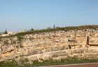
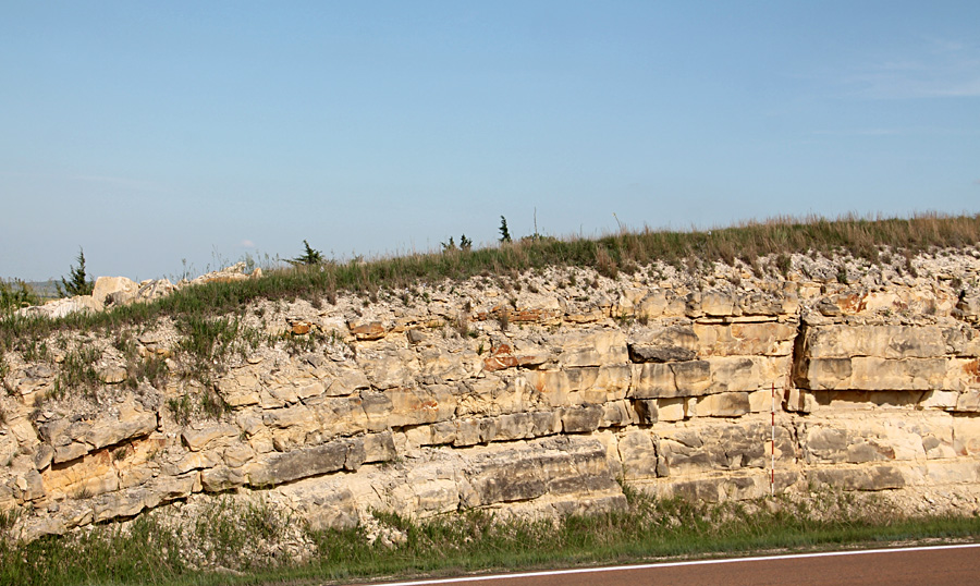
| Figure 4-1 – parallel folding. Gently bent beds of chalky limestone in the Fort Hays Limestone, upper Cretaceous, of western Kansas. Subtle folds of this type are common in areas of stable continental crust. Scale pole on right marked in feet. |
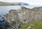
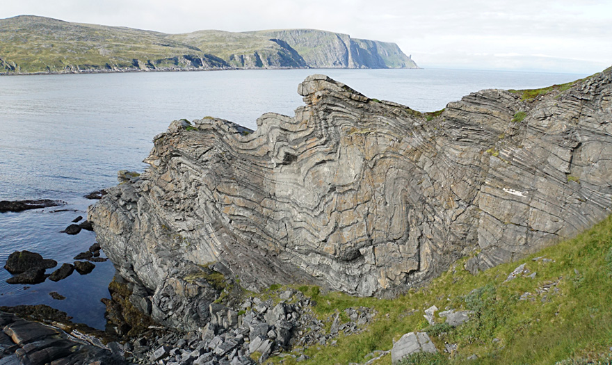
| Figure 4-1 – similar folding. Thickness of beds is stretched and distorted in these strongly folded metamorphic strata in the Caledonian mountain system of Silurian age. Near Kirkeporten, Skarsvĺg, on the island of Magerřya, northernmost Norway.
|
All kinds of rocks display folds: sedimentary and volcanic strata, metamorphic schists and gneisses, granites and other plutonic rocks, salt, glacier ice, and poorly consolidated to unconsolidated materials of all kinds. It should be understood that the conditions under which folding of these rocks took place was probably quite different from what we observe today. For example, many large overturned folds in drift and soft bedrock produced by glacier shoving may have been deformed while in a permafrozen condition.
 Folds in structural geology.
Just as the general attributes of folds vary greatly, so do their origins. The result is that folds of various kinds and sizes are to be found in all sorts of rocks virtually everywhere in the crust of the Earth. Analysis of the geometry and timing of folding may reveal a great deal about the geologic history of a region. Fold geometry may also be economically important, for many mineral and fossil-fuel deposits tend to be locally concentrated in certain portions of folds—oil and natural gas in fold crests, artesian groundwater in fold troughs.
Folds in structural geology.
Just as the general attributes of folds vary greatly, so do their origins. The result is that folds of various kinds and sizes are to be found in all sorts of rocks virtually everywhere in the crust of the Earth. Analysis of the geometry and timing of folding may reveal a great deal about the geologic history of a region. Fold geometry may also be economically important, for many mineral and fossil-fuel deposits tend to be locally concentrated in certain portions of folds—oil and natural gas in fold crests, artesian groundwater in fold troughs.
Geometric elements of folds
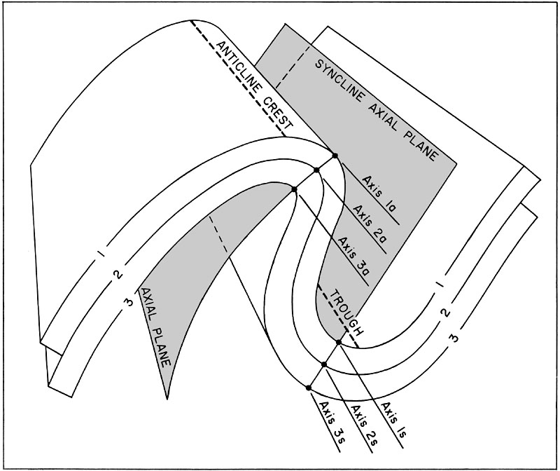
Folds are comprised of linear and planar geometric elements—see Fig. 4-2, and the geometric description of a fold consists of recognizing these elements and measuring their orientations and sizes. Here are the important geometric elements of folds.
- Axis – line of maximum curvature in a folded surface; also called the hinge line.
- Limb – relatively less curved (planar) surface between adjacent axes.
- Crest – line of highest elevation on arch of a folded surface; does not always coincide with the axis.
- Trough – line of lowest elevation on bottom of a folded surface; does not always coincide with the axis.
- Axial plane – a plane which essentially bisects the fold; it is parallel to and contains all axes of folded surfaces; also called the hinge surface.
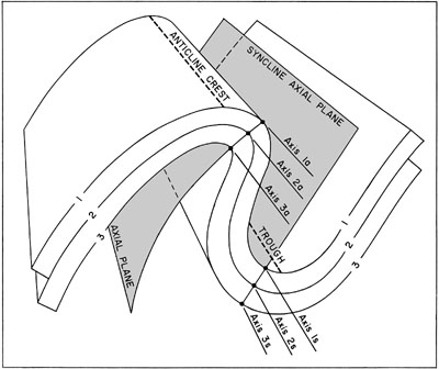
| Figure 4-2. Schematic illustration of the geometric elements of folds. Three folded surfaces (1-3) define a syncline on the right and anticline on the left. The syncline has a flat axial plane, and the anticline has a slighly curved axial plane.
|
The axis and axial surface may be approximated by a line and a plane, although they are not always strictly a straight line or a flat plane. Uparched folds are called anticlines, and down bowed folds are synclines. In Figure 4-2, the anticline on the left displays a gently curved axial plane, and the syncline to the right has a flat axial plane. The tightness of a fold is given by the interlimb angle—see Fig. 4-3, which is simply the angle between the two fold limbs. This angle is measured in a plane perpendicular to the fold axis.
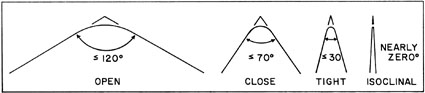 |
| Figure 4-3. Schematic illustration of fold interlimb angle.
|
The axis and axial plane are the two basic geometric elements necessary to describe a fold's orientation. The actual orientation of the fold axis is measured by trend and plunge, and the axial plane is specified by strike and dip. Determination of the other geometric elements of the fold, then, completes the description of the fold's geometry. In the case of small folds that may be seen in their entirety in outcrops, the fold axis and axial plane may often be measured directly. However, this is not always possible, especially with larger folds, and so the axis and axial plane must be determined from measurements of fold limb positions.
The surface outcrop pattern of a fold depends largely on the positions of its axis and axial plane. The typical zig-zag or S-shaped outcrop pattern of plunging folds is illustrated in Figure 4-4, and fold map symbols are shown in Figure 2-2. However, it is not always possible to estimate the axis and axial plane positions based solely on the rock outcrop pattern. Additional information, such as the ages and dips of folded strata, may be necessary to fully interpret the fold position. The outcrop patterns of anticlines and synclines may be distinguished as follows.
- Anticline – strata dip away from the fold center (crest), the oldest rock unit outcrops at the fold center, and the fold plunges toward the closed end of the loop.
- Syncline – strata dip toward the fold center (trough), the youngest rock unit outcrops at the fold center, and the fold plunges toward the open end of the loop.
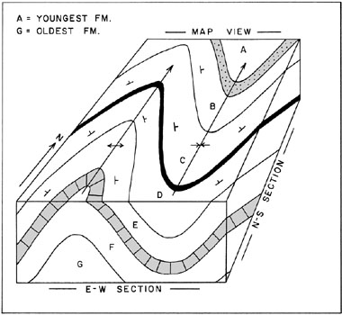
| Figure 4-4. Block diagram showing map and vertical-section views of plunging folds—anticline on left and syncline on right—both plunging northward. See Figure 2-2 for symbols.
|
Fold styles
Fold style refers to the shape and thickness of adjacent layers in a fold. There are two basic styles of folding—see above.
- Parallel – cylindrical or concentric style of folding in which each layer maintains a constant thickness and folded surfaces remain strictly parallel throughout all parts of the fold.
- Similar – style of folding in which adjacent folded surfaces have identical shapes, and layers thicken toward the axial plane and thin in the limbs.
Parallel folds are typical of rocks mildly deformed near the Earth's surface under conditions of relatively low pressure and temperature. Such folds tend to be largely superficial structures that cannot extend deep beneath the surface due to a geometric limitation. Similar folds are characteristic of rocks deformed under conditions of higher pressure and temperature. The thinning of limbs and thickening of the fold core indicate that plastic flowage of rock material took place during deformation. The similar style geometry may be projected upward or downward an infinite distance, because the shape remains constant from layer to layer.
Fold style is a reflection of the competence of rocks during deformation. Competence refers to a rock's strength or foldability. Competent rocks are able to resist the forces of folding to some extent, and so produce open, parallel folds. Incompetent rocks are unable to resist folding, and so form tight, similar or irregular folds. Competence is strictly a relative condition, because rocks which are competent in one situation may behave incompetently in another.
Changes in pressure, temperature, fluid content, or many other factors may cause a change in competence. For example, marble is a competent rock at earth-surface pressure and temperature, but under metamorphic conditions it is quite incompetent. In a stratified sequence of rocks, the competence of layers varies from one to another depending mainly on lithology and thickness. Thus, when the sequence becomes folded, the fold style differs from layer to layer.
Constructing folds
A simple method developed by Busk (1929) for constructing fold cross sections is illustrated in Figure 4-5. The method assumes that the folds are relatively open, do not plunge steeply, and are parallel in style. Dip measurements made at the surface are plotted on a vertical section that is approximately transverse to the trend of the folds.
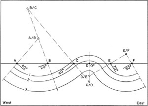
| Figure 4-5. Schematic illustration of constructing folds along a vertical cross section. Strata dip is shown at six sites (A-F) along the section. Folds are constructed in circular arcs; individual layers have uniform thicknesses
across the section.
|
Six dip lines on tilted strata of N-S trending folds are shown at points A-F in the example. Note that the dip angle plotted at each point on the section is the apparent dip of the tilted bed as it appears in the section. Dip measurements need not be from the same stratum, but could be made on any portion of the folds. The folds are constructed by drawing a series of circular arcs that are tangent to the apparent dip lines. Specific steps in this procedure are:
- Calculate the apparent dip of tilted beds at each point on the cross section. Draw in the apparent dip angle for each point; be sure to draw in correct direction of apparent dip.
- Draw construction lines that are perpendicular to each dip line (dashed lines in the example). Adjacent perpendicular construction lines intersect above or below the section. Open circles labelled A/B, B/C, and so on show these intersections in the example.
- Use the intersection points as centers around which to draw arcs between perpendicular construction lines. You need to adjust the radii of arcs for each intersection point. Three folded surfaces formed by arcs drawn in this manner are shown in the example (1-3). Those portions of surfaces 1 and 2 which are above the section between points C and E are shown for completeness, but are not actually present.
Following this method, realistic subsurface folds of parallel style may be constructed and their former position above the land surface could also be projected. However, the folds cannot be constructed more deeply than the shallowest intersection point (in the example D/E). To continue drawing deeper arcs results in a cuspate fold style, which may not be realistic. It is also necessary to have sufficient data points along the section so that no folds are left out of the construction.
Problem
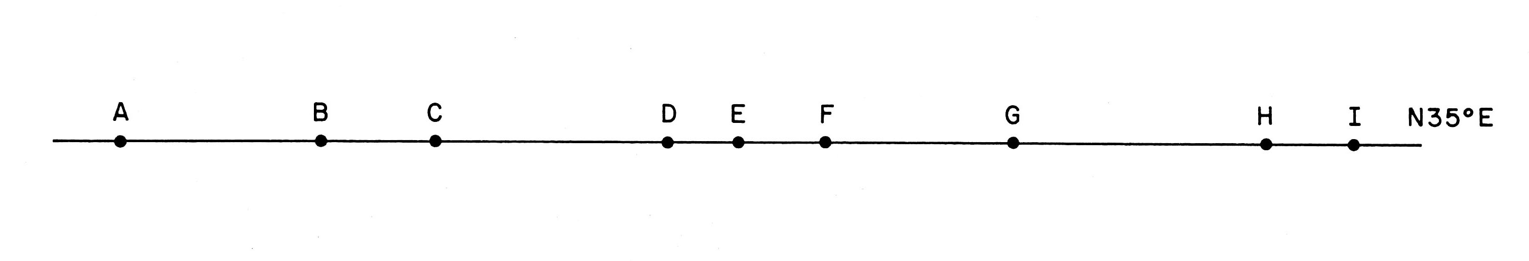
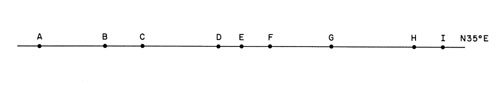
Table 4-1 (below) presents strike-and-dip data for points along the following section—see Fig. 4-6. The section is vertical and strikes (35°) N35E, and folds of the area generally trend NW-SE.
 |
| Figure 4-6. Problem section. Print at full size in landscape format.
|
- Calculate the apparent dip angle and direction in the section at each point; round off apparent dip values to nearest degree.
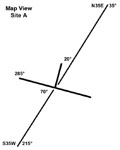
| Example for site A. Map view shows the vertical cross section striking 35-215°. Strike-and-dip symbol: strike = 285°. A = 20° and B = 70°. Use the apparent dip formulas: tan AD = tan TD (40) x cos A (20) or tan AD = tan TD (40) x sin B (70). You should obtain an apparent dip of 38° (NE). Note: apparent dip is always less than true dip and never negative. |
- Following the method outlined above, construct a sequence of parallel folds as deeply beneath the land surface as possible.
- Assuming the section has a horizontal and vertical scale of one inch = one mile, how deeply may the parallel fold geometry of this method be extended before a cuspate style develops?
- From the strike-and-dip data and your fold section, are you able to determine if the folds are plunging; and if so, are they plunging to the NW or SE?
Table 4-1. Strike-and-dip data for tilted strata of section. Strike-and-dip values given according to the right-hand rule.*
| Site | Strike | Dip | | A | 285 | 40 |
| B | horizontal | none |
| C | 155 | 55 |
| D | 130 | 14 |
| E | 295 | 15 |
| F | 270 | 60 |
| G | 265 | 50 |
| H | 280 | 65 |
| I | 130 | 05 |
* Right-hand rule – fingers of the right hand point
downdip, and strike is recorded in the thumb direction.
Reference
- Busk, H.G. 1929. Earth Flexures. Cambridge Univ. Press, Cambridge, England.
5. STRUCTURE CONTOURING
Contour maps
A contour map is an excellent means of showing the geometric configuration of a surface. Topographic maps represent the configuration of the land surface by use of elevation contour lines and spot elevation readings. Hills, valleys, slopes, drainage, and other aspects of the land's topography may be represented and analyzed on typical topographic maps.
In like manner, structure contour maps show the configuration of a rock surface by means of elevation contour lines and spot elevation readings on that surface. Normally, a marker bed, formation boundary, or other distinctive stratigraphic horizon, which is readily recognizible in well logs, seismic sections, or outcrops, could be chosen as the reference surface. Assuming the reference surface was originally flat and horizontal, then any apparent hills or valleys are interpreted as anticlines and synclines, and a sharp drop or rise in elevations may represent a fault.
Structure contour maps are most often employed to display subsurface rocks and structures, but outcrop data may also be used for making such maps. Structural cross sections with different vertical exaggerations may be prepared from structure contour maps, and strike-and-dip measurements may also be made on the reference surface. In short, a thorough structural analysis of the reference surface is possible.
Structure contour maps are especially useful for recognizing epeirogenic structures—gentle warpings, mild folds and small faults developed within the stable craton of the mid-continent region. In this setting, strata are generally near-horizontal with dips of only a few m per km (feet per mile). Such structures are barely recognizible on conventional geologic maps, but are clearly identifible on structure contour maps—see Fig. 5-1. Small contour intervals on maps and large vertical exaggerations (50 to 300 times) on cross sections could be employed to emphasize otherwise subtle structures. Structure contour mapping is a standard approach for subsurface geological evaluation of oil and gas fields, groundwater aquifers, and other economic deposits.
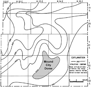
| Figure 5-1. Structure contour map on the base of the Kansas City Group (upper Pennsylvanian) for a portion of Linn County, eastern Kansas. The Mound City Dome is an anticline with closure at 1000 feet elevation. Dip of bedrock around the dome is only 1-2°. Each full township measures 6 by 6 miles. Adapted from Seevers (1969).
|
Contouring technique
Figure 5-2 shows maps of elevation control points on a structural surface and the resulting elevation contours of the surface. Each contour represents a line of constant (equal) elevation on that surface. In some cases, elevation control points are exactly equal to the contour lines, but elsewhere the positions of contours are interpolated between adjacent control points.
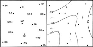
| Figure 5-2. Maps of elevation control points (left) and contour lines (right) on a structural surface. The map area represents one section (one square mile); elevations given in feet; strike-and-dip symbols shown on contour map.
|
However, the exact positions of contour lines between control points cannot be definitely known. Examine the relationship between control-point and contour-line elevations in this example. Here are some basic rules to follow in constructing contour maps.
- Contours are generally separate, smooth lines that are more-or-less parallel to each other.
- A single contour line never branches or divides.
- Contours may form closed loops around domes or basins. Tick marks are used to indicate a closed depression.
- Aside from closed loops, each contour should extend to the map edges; contours cannot simply begin or end in the middle of the map.
- Adjacent contour lines may merge only at vertical cliffs or faults which offset the surface.
- Use a contour interval that is appropriate to the elevation range present.
Structure contour maps clearly reveal any folds present in the reference surface. For example, an open anticline plunging gently to the northeast is visible in Figure 5-2. Appropriate fold and fault symbols may be shown directly on the map. Strike and dip at any point on the surface could be determined easily—strike is parallel and dip is perpendicular to contour lines. The dip angle may also be measured.
Consider the two points along the western edge of the map (fig. 5-2) at elevations of 84 and 116 feet. A straight line drawn between these two points is approximately perpendicular to the contours, and so represents a true dip line. The two points are 4150 feet apart and 32 feet different in elevation. Applying the dip-angle formula of Exercise 2: 32/4150 = tan (dip angle); dip angle = 0.4° N, or 41 feet per mile (one mile = 5280 feet). This shallow dip is quite typical of epeirogenic structures.
Several computer programs have been developed for routine contouring of structural data. Often a given set of control-point elevations could be contoured in several quite different configurations. The computer program normally would contour the simplist possible solution. Nonetheless, there are still many situations where manual contouring by an experienced geologist is preferable. The geologist should recognize this and decide on the best interpretation based on additional surface or subsurface information.
Problem
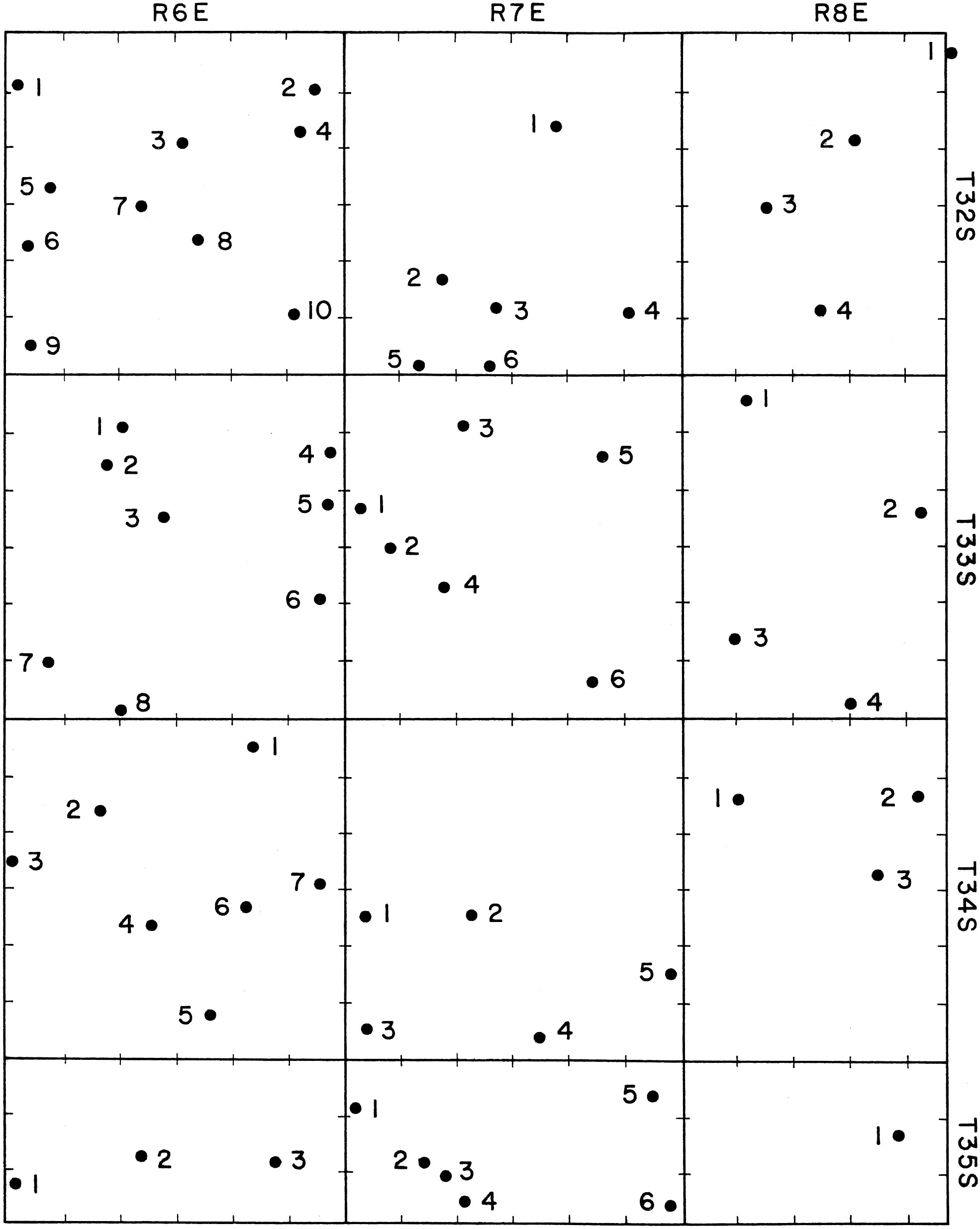
In this exercise you will prepare a structure contour map of Paleozoic strata in the Flint Hills of Cowley County, south-central Kansas. The locations of 63 well-holes are shown on the accompanying map—see Fig. 5-3. The map displays township-and-range boundaries for the southeastern portion of Cowley County. Six whole and six partial townships are covered by the map. A full township measures 6 miles on a side and is divided into 36 sections.
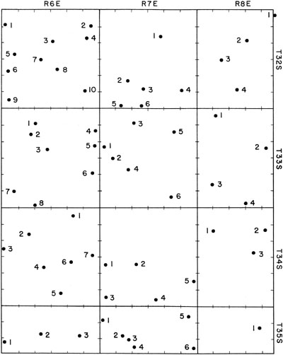
| Figure 5-3. Map of townships and well locations in southeastern Cowley County, Kansas. Adapted from Bayne (1962, plate 5). Print this map at full size for the exercise.
|
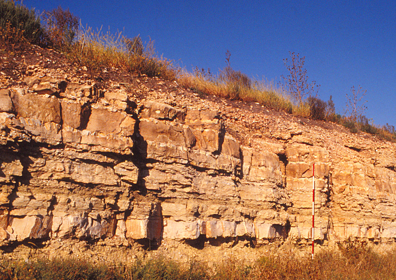
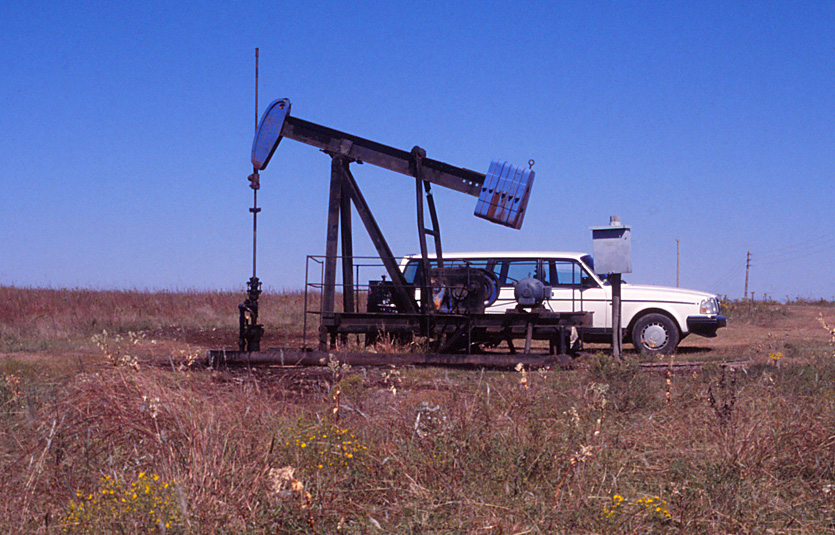
Upper Pennsylvanian and lower Permian limestone and shale crop out at the surface throughout the area shown. The general regional dip of these strata at the surface averages 25 feet per mile (~0.3°) westward. The most pronounced structural anomaly at the surface is the Dexter Anticline, which trends north and northeast across the map area. Surface strata dip eastward more than 100 feet within half a mile (dip >2°) east of the anticline's crest, but on the western flank of the anticline the dip is only about half as steep. Many producing oil and gas wells have been drilled in association with this and other similar structures of the region—see Fig. 5-4.
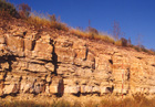
| Figure 5-4. Road cut in the Florence Limestone (lower Permian) in the southern Flint Hills (left). Limestone with interbedded chert nodules and layers. Scale pole is marked in feet. Shinn NE oil field (right), located on the Beaumont anticline in southeastern Butler County. These examples are similar to the problem area in Cowley County.
| 
|
Contours on the top of the Douglas Group (subsurface Pennsylvanian) show more structural relief than do contours on surface rocks, but they more nearly reflect surface structures than would contours on any deeper formations. Table 5-1 gives elevations in feet on the top of the Douglas Group for each township in the map area.
- Prepare a structure contour map on the top of the Douglas Group for Figure 5-3. Use a 50-foot contour interval (50, 0, -50, -100, etc.). Assume there are no faults present.
- Prepare a structural cross section (profile) running E-W through point 4, T33S/R7E. Use a vertical scale of one inch = 200 feet.
- Determine the map scale, and calculate the vertical exaggeration of your section. Hint: divide the horizontal (map) scale by the vertical (section) scale. Note: both scales must be in the same units or fractions.
- Describe the regional strike and dip evident on your map. Calculate the actual dip between point 6, T33S/R7E, and point 4, T33S/R8E.
- Place appropriate fold symbols on your contour map. Do you find any subsurface evidence for the Dexter Anticline? If so, describe the subsurface expression of the anticline.
- There are multiple ways to configure the structure contours on the basis of the available subsurface data. Use dashed lines or colored lines to show alternate contour lines and fold symbols.
- Do any of your contour versions represent significantly different structures? Which contour version do you prefer based on information about surface structures?
Table 5-1. Elevations on the top of the Douglas Group (see map). Adapted from Bayne (1962, plate 5).
Township
and Range | Well | Elev. |
T32S/R6E | 1 | -329 |
| | 2 | -127 | | | 3 | -296 |
| | 4 | -185 | | | 5 | -315 | | | 6 | -351 |
| | 7 | -310 | | | 8 | -280 |
| | 9 | -331 | | | 10 | -270 | |
Township
and Range | Well | Elev. | T32S/R7E | 1 | - 28 |
| | 2 | -110 |
| | 3 | - 20 |
| | 4 | - 46 |
| | 5 | -117 |
| | 6 | - 51 |
T32S/R8E | 1 | 140 | | | 2 | 88 |
| | 3 | 40 | | | 4 | 83 | | |
Township
and Range | Well | Elev. | T33S/R6E | 1 | -332 | | | 2 | -355 |
| | 3 | -355 |
| | 4 | -156 | | | 5 | -135 |
| | 6 | -59 |
| | 7 | -365 |
| | 8 | -375 | |
Township
and Range | Well | Elev. | T33S/R7E | 1 | -55 |
| | 2 | -175 |
| | 3 | -54 |
| | 4 | -182 |
| | 5 | -38 | | | 6 | -14 |
T33S/R8E | 1 | 50 | | | 2 | 160 | | | 3 | 100 | | | 4 | 191 | | |
Township
and Range | Well | Elev. | T34S/R6E | 1 | -180 |
| | 2 | -250 | | | 3 | -362 |
| | 4 | -240 | | | 5 | -233 |
| | 6 | -145 | | | 7 | -80 | |
Township
and Range | Well | Elev. | T34S/R7E | 1 | -147 |
| | 2 | -58 |
| | 3 | -150 |
| | 4 | 18 |
| | 5 | 80 |
T34S/R8E | 1 | 90 | | | 2 | 215 |
| | 3 | 120 | | |
Township
and Range | Well | Elev. | T35S/R6E | 1 | -257 |
| | 2 | -256 |
| | 3 | -225 |
T35S/R7E | 1 | -191 | | | 2 | -140 |
| | 3 | -120 |
| | 4 | -85 |
| | 5 | 115 |
| | 6 | 35 |
T35S/R8E | 1 | 200 | | | |
References
- Bayne, C.K. 1962. Geology and ground-water resources of Cowley County, Kansas. Kansas Geological Survey, Bulletin 158.
- Seevers, W.J., 1969. Geology and ground-water resources of Linn County, Kansas. Kansas Geological Survey, Bulletin 193, 62 p.
6. EQUAL-ANGULAR STEREONET
Stereographic projections
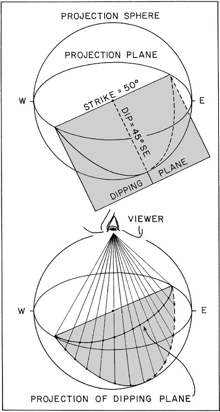
A stereographic projection, or more simply a stereonet, is a powerful method for displaying and manipulating the 3-dimensional geometry of lines and planes. The orientations of lines and planes may be plotted relative to the center of a sphere, called the projection sphere, as shown at the top of Figure 6-1. The intersection made by the line or plane with the sphere's circumference defines the 3-dimensional orientation of the line or plane. The projection sphere is divided in half by a horizontal plane called the projection plane. Compass directions are indicated on the projection plane. All measurements are made relative to horizontal, so only the lower hemisphere of the projection sphere need be used.
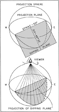
| Figure 6-1. Dipping plane plotted relative to the center of a projection sphere (above), and horizontal projection of that plane (below).
|
The lower stereonet hemisphere may be projected in various manners onto a flat graph. However, stereographic projections distort the distances and spatial relationships of features. Stereonets are preferable to maps or cross sections for solving many geometric problems involving lines and planes that are common in structural geology. Two popular stereographic projections are: (1) the equal-angular or Wulff stereonet, and (2) the equal-area or Schmidt stereonet.
For further information, see Stereonet 11.
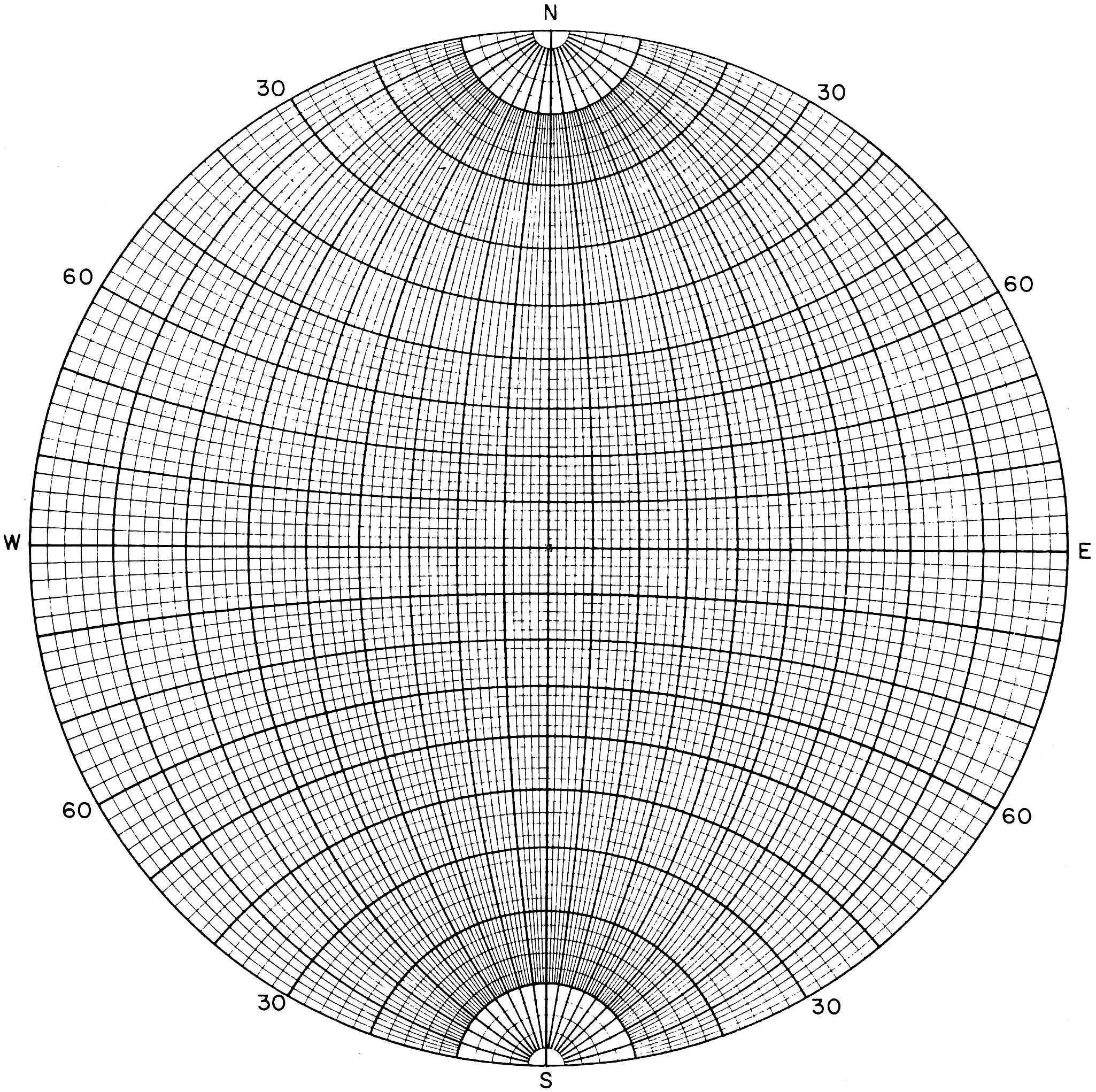
Wulff stereonet
The Wulff stereonet is perhaps the easier of the two projections to visualize, and so we will examine it first. Imagine that your eye is positioned at the zenith of the projection sphere (Fig. 6-1). The dipping plane intersects the lower hemisphere forming an arc that your eye visualizes on the horizontal projection plane. The resulting projection-plane arc is, in effect, a single-point perspective view of the dipping plane as seen from the top of the sphere. This method of projection is the basis of the Wulff stereonet—see Fig. 6-2.
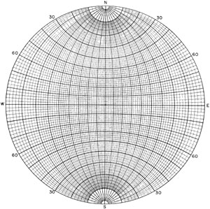
| Figure 6-2. Wulff stereographic projection. Print out a full-sized version for the examples below and problem.
|
The Wulff stereonet consists of a series of circular arcs that form meridians running N-S and parallels running E-W. Although the meridians and parallels resemble longitude and latitude lines on a map, they are not; the stereonet is not
a map. The meridians represent N-S striking planes with dips ranging from 0 to 90° east and west. Angles are preserved on the Wulff stereonet; note that meridians and parallels always intersect at right angles. However, size and shape are distorted, as
seen by comparing different portions of the projection. Lines and planes plot on the Wulff stereonet as follows—see Fig. 6-3.
- Vertical line – single point at exact center.
- Plunging line – single point, closer to center for steeper plunge, closer to edge for shallower plunge.
- Horizontal line – two "half points" on opposite sides.
- Vertical plane – straight line through center.
- Dipping plane – circular arc, closer to center for steep dip, closer to edge for shallower dip.
- Horizontal plane – great circle that coincides with outer edge of stereonet.
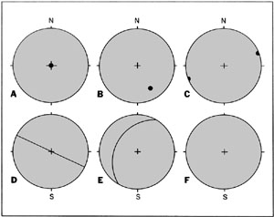
| Figure 6-3. Representative stereonet plots of lines and planes: A - vertical line, B - plunging line (trend/plunge = 150/20°), C - horizontal line (trend = 70°), D - vertical plane (strike = 115°), E - dipping plane (strike/dip = 210/30°), F - horizontal plane (coincides with outer edge of stereonet).
|
Plotting lines and planes
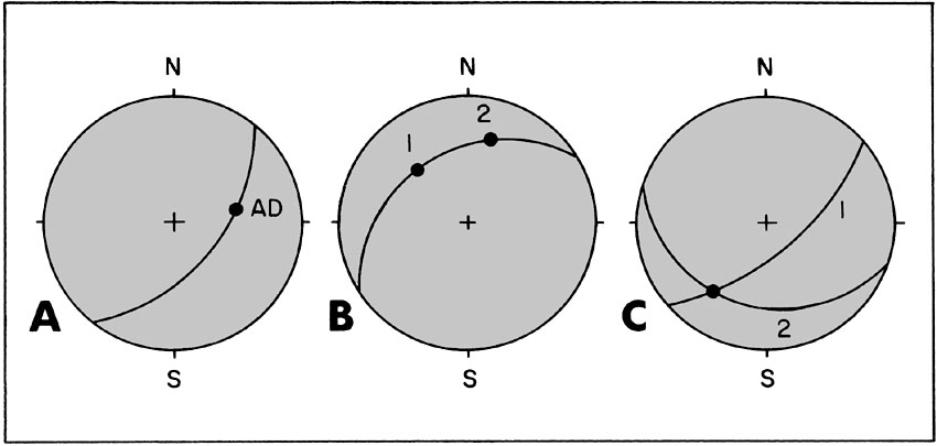
The traditional procedure in making stereonet plots is to work on tracing paper laid over the stereonet. A thumbtack is pushed through the stereonet from the back side, so that the point sticks up in the center of the stereonet. A sheet of tracing paper is then pushed down on the thumbtack, so as to rotate around the center of the stereonet. Plastic stereonet templates and computer programs are also available for stereographic analysis. In either case, once the tracing paper is positioned, be sure to mark the north, south, east, and west points as reference marks on the outer edge of the stereonet. You are now ready to begin plotting lines and planes. Work through the three following examples to learn how to use the Wulff stereonet—see Fig. 6-4.
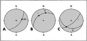
| Figure 6-4. Stereonet plots illustrating examples A, B, and C discussed below.
|
Example A: Plot a plane which has a strike of 40° and a dip angle of 50°. Note: following the right-hand rule means that dip direction is 90° clockwise from strike; in this case strike is to the northeast and dip direction is toward the southeast. What is the apparent dip angle of the plane for an apparent dip line that trends 80°?
- To plot a plane first mark the strike along the outer edge of the stereonet, and then add 90° and mark the dip trend along the outer edge of the stereonet. In this example, you should mark 40° (strike) and 130° (SE dip).
Note: for planar strike-and-dip values, the right-hand rule is assumed. The fingers of the right hand point downdip on the plane, and the strike is recorded for the thumb direction. Always follow this rule to avoid mistakes.
- Now rotate the tracing so that your strike mark points straight north. This brings your dip mark onto the E-W axis of the stereonet. All dip or plunge angles are measured on the E-W axis.
- Count the dip angle inward from your dip mark along the E-W axis; in this case count in 50°. Draw in the N-S meridian arc which crosses the E-W axis at the dip angle you counted.
- Finally, rotate the tracing back to its original position; the arc represents a plane with strike = 40° and dip angle = 50°.
- To find the apparent dip, mark the trend of 80° on the outer edge of the stereonet.
- Rotate the apparent-dip-trend mark at 80° to the E-W axis, and count the plunge angle inward along the E-W axis to the spot where the arc crosses the axis. Mark that point. You should count an apparent dip angle of 38° in this example. Use the apparent dip formulas to confirm your graphical answer.
Example B: Find the true strike and dip of a plane given the following two apparent dips: (1) trend/plunge = 315/30°, and (2) trend/plunge = 14/22°.
- You need to plot two points for the two (linear) apparent dips. Begin by marking each trend on the outer edge of the stereonet.
- Rotate the tracing so that trend 1 is on the E-W axis, and count inward 30°. Mark that point for apparent dip 1.
- Rotate the tracing so that trend 2 is on the E-W axis, and count inward 22°. Mark that point for apparent dip 2. You should now have marked two points.
- Now rotate the tracing so that both points fall on the same N-S circular arc, and sketch in that arc. This arc represents the plane in question.
- Without moving the tracing, count inward along the E-W axis to the arc to determine the plane's true dip.
- Finally, rotate the tracing back to its original position and determine the strike of the arc where its ends meet the outer edge of the stereonet. You should have a plane whose strike/dip = 237/30°. Remember to use the right-hand rule.
Example C: Find the trend and plunge of the line formed by the intersection of the following two planes: (1) strike/dip = 50/60° and (2) strike/dip = 110/20°. Determine the angle between the two planes.
- Plot arcs for both planes following the procedure of example A. For each plane, mark the dip line (90° clockwise from strike) as a point. After rotating the tracing back to its original position, you should obtain two arcs.
- Mark the point at which the arcs intersect each other. This point represents the intersection line of the two planes. The compass direction (trend) of the point is determined along the outer edge of the stereonet; in this case, trend = 219°.
- Now rotate the intersection point to the E-W axis, and count the plunge angle inward along the axis to the point. You should obtain a plunge of 19° in this example.
- Now, rotate the tracing so that the two dip points fall on the same N-S meridian. Count the angle between these two points; it equals the angle between the two planes, 52° in this case.
As these examples demonstrate, it is possible to quickly solve geometric problems on the stereonet that would otherwise be difficult to calculate. The stereonet is a graphical technique, so it is only as accurate as your sketching of lines and points on it. Do not expect answers from the paper stereonet that are closer than +1°. This level of precision is more than suitable for most problems in structural geology. Proficiency with the stereonet requires practice, therefore it is strongly recommended that you work through the previous examples—either on paper or with Stereonet 11 (or both)—before attempting to solve the problem.
Problem
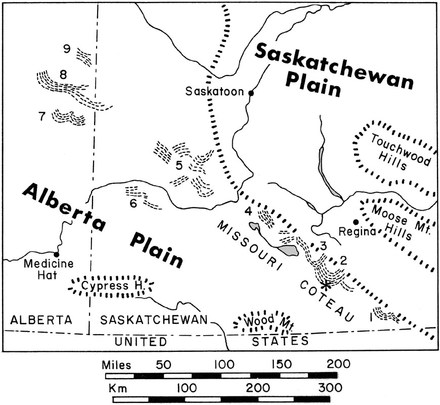
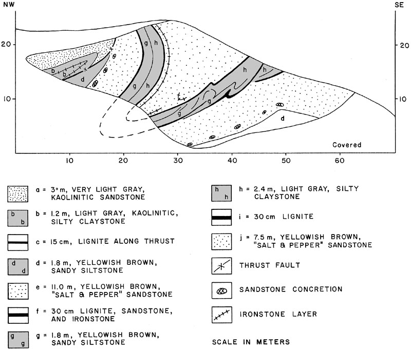
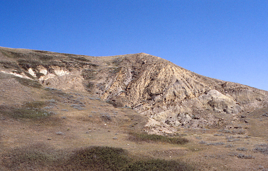
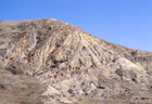
The Dirt Hills and Cactus Hills of southern Saskatchewan are among the largest ice-pushed hills in the world—see Fig. 6-5. A large natural exposure on the southern side of the Dirt Hills displays deformed bedrock of the Whitemud and lower Ravenscrag Formations—see Fig. 6-6. Lower Ravenscrag strata normally rest on top of the Whitemud Formation, but here the stratigraphy is upset. A tight fold of Whitemud strata (beds a-b) is thrust over a large, overturned fold of lower Ravenscrag sediments (beds d-j) along a thin seam of lignite (unit c).

| Figure 6-5. Major ice-shoved hills of southern Saskatchewan and adjacent Alberta (numbered sites). 2 = Dirt Hills; 3 = Cactus Hills. Dashed lines indicate general trends of ice-shoved ridges. Location of exposure in southern Dirt Hills indicated by asterisk. Adapted from Kupsch (1962, fig.1).
|
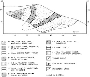
| Figure 6-6. Measured section of exposure, southern Dirt Hills, Saskatchewan. Whitemud strata are beds a-b; Ravenscrag strata are beds d-j. No vertical exaggeration; adapted from Aber (1993).
|
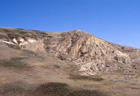
| Large folds on the southern flank of the Dirt Hills, southern Saskatchewan, Canada. Overview (left) showing an exposure of Whitemud Formation (white, upper left) thrust over lower Ravenscrag Formation (brown, center). The normal stratigraphy is inverted, and both formations are strongly folded. Close-up view of large, overturned fold of the lower Ravenscrag Formation (right). Compare with measured section (above).
| 
|
The Whitemud fold axis was measured directly in the field—trend/plunge = 110/15°. However, the axis of the larger Ravenscrag fold was covered and could not be measured directly. The upper limb of the Ravenscrag fold strikes/dips 284/70°; its lower limb strikes/dips 284/46°. You may use the large (paper) Wulff stereonet or Stereonet 11 to answer the following questions.
- Plot the two Ravenscrag fold limbs (planar) on the stereonet. The intersection of the two planes represents the fold axis. What are the trend and plunge of the fold axis?
- Plot the Whitemud fold axis (linear) on the same stereonet. Are the two fold axes approximately parallel? Do the fold axes correspond to the local trend of the Dirt Hills?
- What is the angle between the limbs of the Ravenscrag fold?
- Based on your analysis of this exposure, what was the local direction of ice shoving that created these structures?
References
- Aber, J.S. 1993. Glaciotectonic landforms and structures. In Sauchyn, D.J. (ed.), Quaternary and Late Tertiary landscapes of southwestern Saskatchewan and adjacent areas. Canadian Plains Research Center, Canadian Plains Proceedings 25, vol. 2, p. 20-26. Regina, Canada.
- Kupsch, W. O. 1962. Ice-thrust ridges in western Canada. Journal of Geology 70, p. 582-594.
 Return to Table of Contents.
Notice: This course was prepared for the use and benefit of students enrolled at Emporia State University. Others are welcome to view the course webpages. Any other use of text, imagery or curriculum materials is prohibited without permission. © J.S. Aber (2021).
Return to Table of Contents.
Notice: This course was prepared for the use and benefit of students enrolled at Emporia State University. Others are welcome to view the course webpages. Any other use of text, imagery or curriculum materials is prohibited without permission. © J.S. Aber (2021).